
I always say that learning linear regression in Python is the best first step towards machine learning. Linear regression is simple and easy to understand even if you are relatively new to data science. So spend time on 100% understanding it! If you get a grasp on its logic, it will serve you as a great foundation for more complex machine learning concepts in the future.
In this tutorial, I’ll show you everything you’ll need to know about it: the mathematical background, different use-cases and most importantly the implementation. We will do that in Python — by using numpy (polyfit).
Note: This is a hands-on tutorial. I highly recommend doing the coding part with me! If you haven’t done so yet, you might want to go through these articles first:
- How to install Python, R, SQL and bash to practice data science!
- Python libraries and packages for Data Scientists
- Learn Python from Scratch
Download the code base!
Find the whole code base for this article (in Jupyter Notebook format) here:
Linear Regression in Python (using Numpy polyfit)
Download it from: here.
The mathematical background
Remember when you learned about linear functions in math classes?
I have good news: that knowledge will become useful after all!
Here’s a quick recap!
For linear functions, we have this formula:
y = a*x + b
In this equation, usually, a and b are given. E.g:
a = 2
b = 5
So:
y = 2*x + 5
Knowing this, you can easily calculate all y values for given x values.
E.g.
when x is… | y is… |
| 0 | 2*0 + 5 = 5 |
| 1 | 2*1 + 5 = 7 |
| 2 | 2*2 + 5 = 9 |
| 3 | 2*3 + 5 = 11 |
| 4 | 2*4 + 5 = 13 |
…
If you put all the x–y value pairs on a graph, you’ll get a straight line:
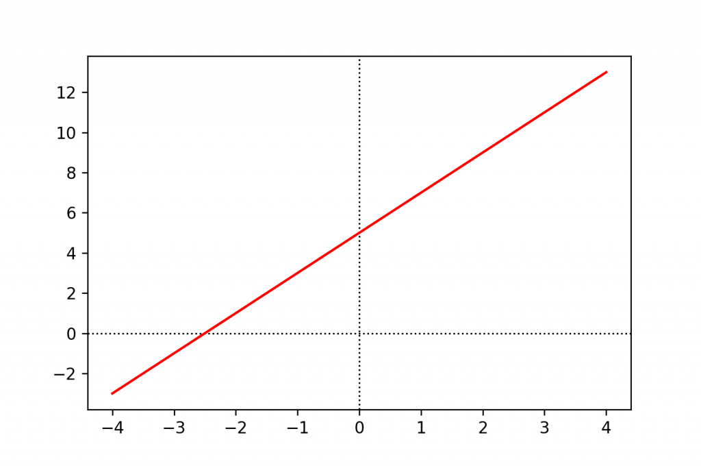
The relationship between x and y is linear.
Using the equation of this specific line (y = 2 * x + 5), if you change x by 1, y will always change by 2.
And it doesn’t matter what a and b values you use, your graph will always show the same characteristics: it will always be a straight line, only its position and slope change. It also means that x and y will always be in linear relationship.
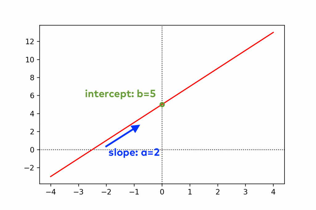
In the linear function formula:
y = a*x + b
- The
avariable is often called slope because – indeed – it defines the slope of the red line. - The
bvariable is called the intercept.bis the value where the plotted line intersects the y-axis. (Or in other words, the value ofyisbwhenx = 0.)
This is all you have to know about linear functions for now…
But why did I talk so much about them?
Because linear regression is nothing else but finding the exact linear function equation (that is: finding the a and b values in the y = a*x + b formula) that fits your data points the best.
Note: Here’s some advice if you are not 100% sure about the math. The most intuitive way to understand the linear function formula is to play around with its values. Change the a and b variables above, calculate the new x-y value pairs and draw the new graph. Repeat this as many times as necessary. (Tip: try out what happens when a = 0 or b = 0!) By seeing the changes in the value pairs and on the graph, sooner or later, everything will fall into place.
A typical linear regression example
Machine learning – just like statistics – is all about abstractions. You want to simplify reality so you can describe it with a mathematical formula. But to do so, you have to ignore natural variance — and thus compromise on the accuracy of your model.
If this sounds too theoretical or philosophical, here’s a typical linear regression example!
We have 20 students in a class and we have data about a specific exam they have taken. Each student is represented by a blue dot on this scatter plot:
- the X axis shows how many hours a student studied for the exam
- the Y axis shows the scores that she eventually got

E.g. she studied 24 hours and her test result was 58%:
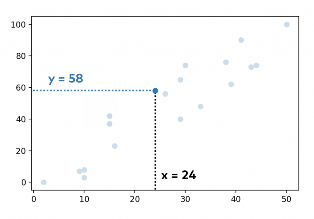
We have 20 data points (20 students) here.
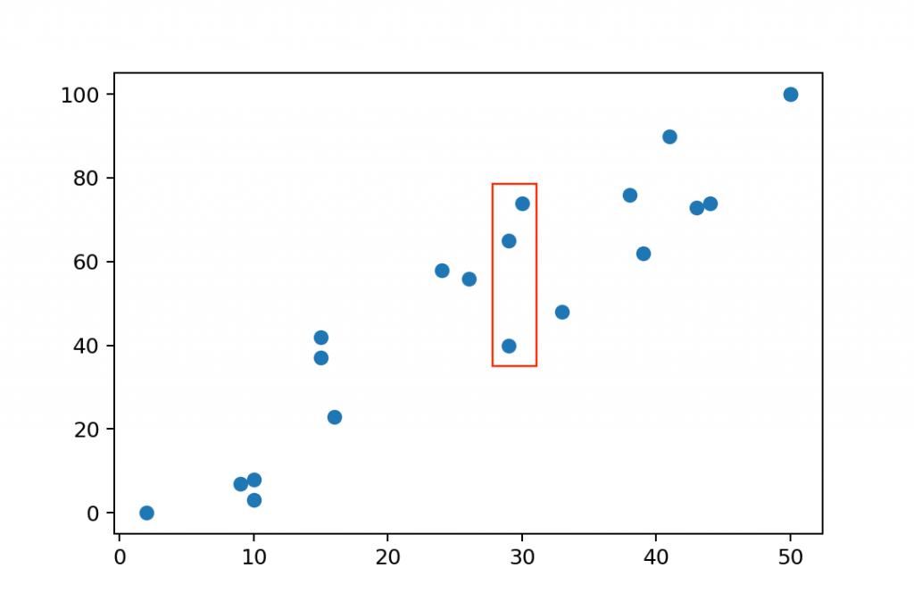
By looking at the whole data set, you can intuitively tell that there must be a correlation between the two factors. If one studies more, she’ll get better results on her exam. But you can see the natural variance, too. For instance, these 3 students who studied for ~30 hours got very different scores: 74%, 65% and 40%.
Anyway, let’s fit a line to our data set — using linear regression:
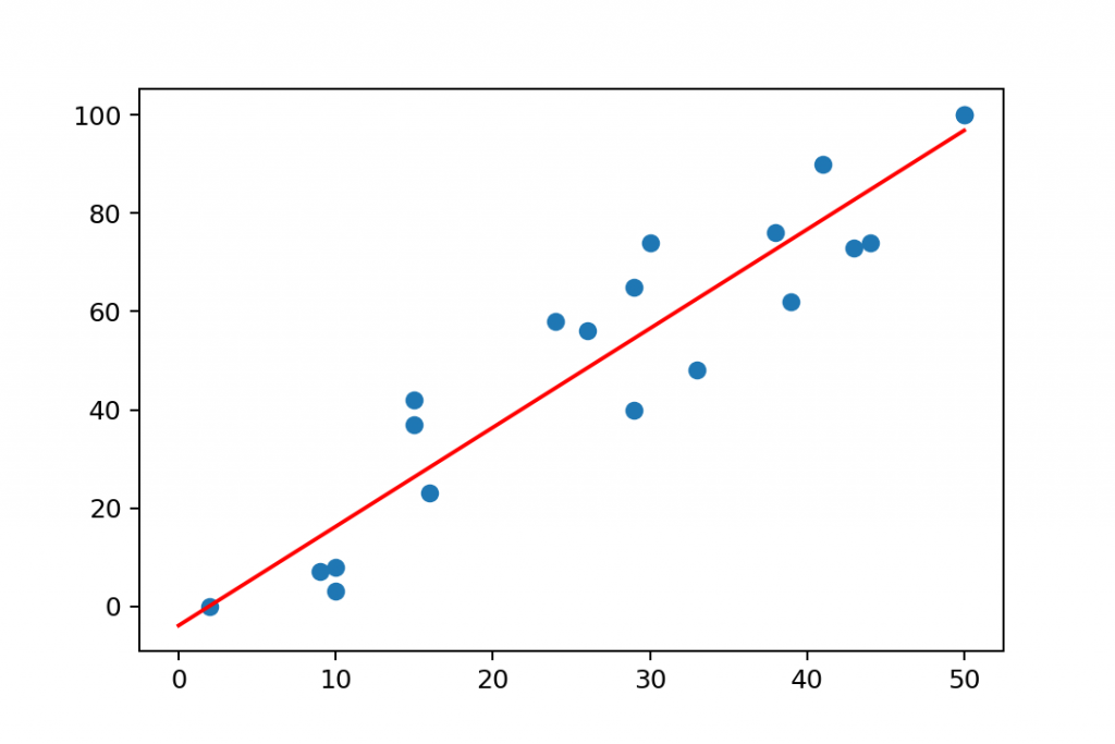
Nice, we got a line that we can describe with a mathematical equation – this time, with a linear function. The general formula was:
y = a * x + b
And in this specific case, the a and b values of this line are:
a = 2.01
b = -3.9
So the exact equation for the line that fits this dataset is:
y = 2.01*x - 3.9
And how did I get these a and b values? By using machine learning.
If you know enough x–y value pairs in a dataset like this one, you can use linear regression machine learning algorithms to figure out the exact mathematical equation (so the a and b values) of your linear function.
Linear regression terminology
Before we go further, I want to talk about the terminology itself — because I see that it confuses many aspiring data scientists. Let’s fix that here!
Okay, so one last time, this was our linear function formula:
y = a*x + b
The a and b variables:
The a and b variables in this equation define the position of your regression line and I’ve already mentioned that the a variable is called slope (because it defines the slope of your line) and the b variable is called intercept.
In the machine learning community the a variable (the slope) is also often called the regression coefficient.
The x and y variables:
The x variable in the equation is the input variable — and y is the output variable.
This is also a very intuitive naming convention. For instance, in this equation:
y = 2.01*x - 3.9
If your input value is x = 1, your output value will be y = -1.89.
But in machine learning these x-y value pairs have many alternative names… which can cause some headaches. So here are a few common synonyms that you should know:
- input variable (
x) – output variable (y) - independent variable (
x) – dependent variable (y) - predictor variable (
x) – predicted variable (y) - feature (
x) – target (y)
See, the confusion is not an accident… But at least, now you have your linear regression dictionary here.
How does linear regression become useful?
Having a mathematical formula – even if it doesn’t 100% perfectly fit your data set – is useful for many reasons.
- Predictions: Based on your linear regression model, if a student tells you how much she studied for the exam, you can come up with a pretty good estimate: you can predict her results even before she writes the test. Let’s say someone studied
20hours; it means that her predicted test result will be2.01 * 20 - 3.9 = 36.3. - Outliers: If something unexpected shows up in your dataset – someone is way too far from the expected range…
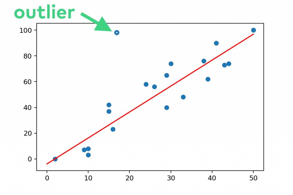
… let’s say, someone who studied only 18 hours but got almost 100% on the exam… Well, that student is either a genius — or a cheater. But she’s definitely worth the teachers’ attention, right? 🙂 By the way, in machine learning, the official name of these data points is outliers.
And both of these examples can be translated very easily to real life business use-cases, too!
Predictions are used for: sales predictions, budget estimations, in manufacturing/production, in the stock market and in many other places. (Although, usually these fields use more sophisticated models than simple linear regression.)
Finding outliers is great for fraud detection. And it’s widely used in the fintech industry. (E.g. preventing credit card fraud.)
The limitations of machine learning models
It’s good to know that even if you find a very well-fitting model for your data set, you have to count on some limitations.
Note: These are true for essentially all machine learning algorithms — not only for linear regression.
Limitation #1: a model is never a perfect fit
As I said, fitting a line to a dataset is always an abstraction of reality. Describing something with a mathematical formula is sort of like reading the short summary of Romeo and Juliet. You’ll get the essence… but you will miss out on all the interesting, exciting and charming details.
Similarly in data science, by “compressing” your data into one simple linear function comes with losing the whole complexity of the dataset: you’ll ignore natural variance.
But in many business cases, that can be a good thing. Your mathematical model will be simple enough that you can use it for your predictions and other calculations.
Note: One big challenge of being a data scientist is to find the right balance between a too-simple and an overly complex model — so the model can be as accurate as possible. (This problem even has a name: bias-variance tradeoff, and I’ll write more about this in a later article.)
But a machine learning model – by definition – will never be 100% accurate.
Limitation #2: you can’t go beyond the range of your historical data
Many data scientists try to extrapolate their models and go beyond the range of their data.
For instance, in our case study above, you had data about students studying for 0-50 hours. The dataset hasn’t featured any student who studied 60, 80 or 100 hours for the exam. These values are out of the range of your data. If you wanted to use your model to predict test results for these “extreme” x values… well you would get nonsensical y values:
E.g. your model would say that someone who has studied x = 80 hours would get:
y = 2.01*80 - 3.9 = 159% on the test.
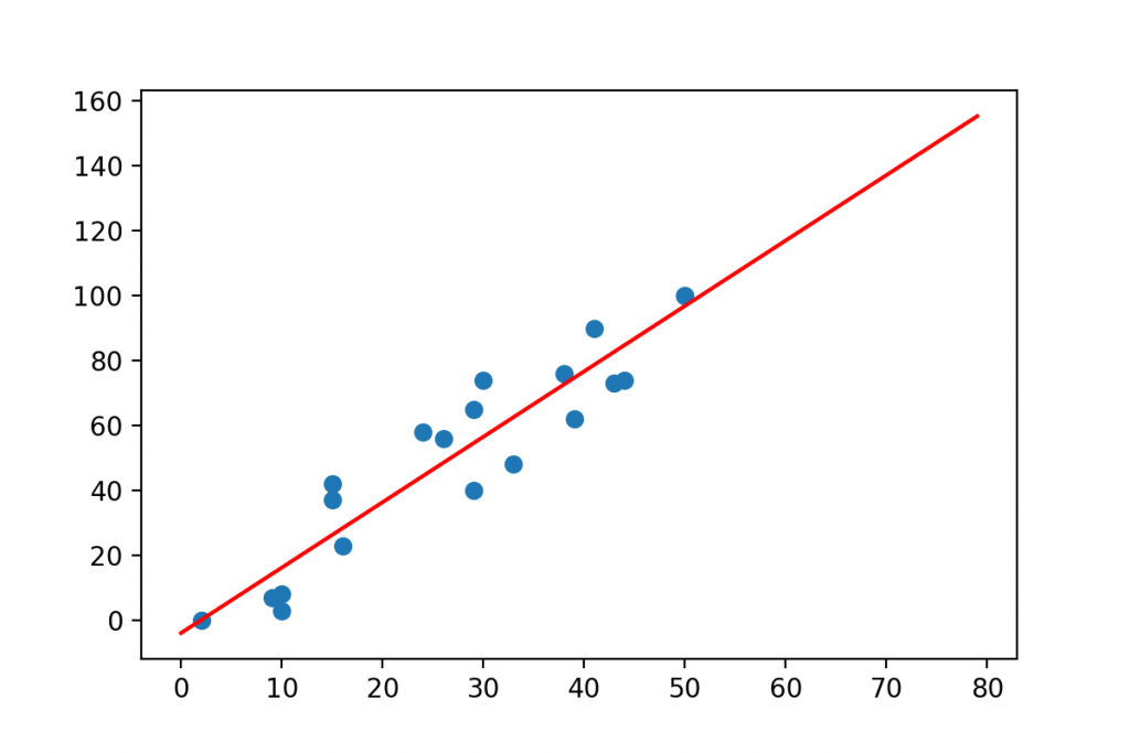
…but 100% is the obvious maximum, right?
The point is that you can’t extrapolate your regression model beyond the scope of the data that you have used creating it. Well, in theory, at least...
Because I have to admit, that in real life data science projects, sometimes, there is no way around it. If you have data about the last 2 years of sales — and you want to predict the next month, you have to extrapolate. Even so, we always try to be very careful and don’t look too far into the future. The further you get from your historical data, the worse your model’s accuracy will be.
Linear Regression in Python
Okay, now that you know the theory of linear regression, it’s time to learn how to get it done in Python!
Let’s see how you can fit a simple linear regression model to a data set!
Well, in fact, there is more than one way of implementing linear regression in Python. Here, I’ll present my favorite — and in my opinion the most elegant — solution. I’ll use numpy and its polyfit method.
We will go through these 6 steps:
- Importing the Python libraries we will use
- Getting the data
- Defining
xvalues (the input variable) andyvalues (the output variable) - Machine Learning: fitting the model
- Interpreting the results (coefficient, intercept) and calculating the accuracy of the model
- Visualization (plotting a graph)
Note: You might ask: “Why isn’t Tomi using sklearn in this tutorial?” I know that (in online tutorials at least) Numpy and its polyfit method is less popular than the Scikit-learn alternative… true. But in my opinion, numpy‘s polyfit is more elegant, easier to learn — and easier to maintain in production! sklearn‘s linear regression function changes all the time, so if you implement it in production and you update some of your packages, it can easily break. I don’t like that. Besides, the way it’s built and the extra data-formatting steps it requires seem somewhat strange to me. In my opinion, sklearn is highly confusing for people who are just getting started with Python machine learning algorithms. (By the way, I had the sklearn LinearRegression solution in this tutorial… but I removed it. That’s how much I don’t like it. So trust me, you’ll like numpy + polyfit better, too. :-))
Linear Regression in Python – using numpy + polyfit
Fire up a Jupyter Notebook and follow along with me!
Note: Find the code base here and download it from here.
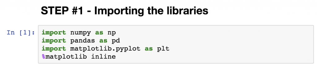
STEP #1 – Importing the Python libraries
Before anything else, you want to import a few common data science libraries that you will use in this little project:
numpypandas(you will store your data in pandas DataFrames)matplotlib.pyplot(you will usematplotlibto plot the data)
Note: if you haven’t installed these libraries and packages to your remote server, find out how to do that in this article.
Start with these few lines:
import numpy as np
import pandas as pd
import matplotlib.pyplot as plt
%matplotlib inline
(The %matplotlib inline is there so you can plot the charts right into your Jupyter Notebook.)
To be honest, I almost always import all these libraries and modules at the beginning of my Python data science projects, by default. But apart from these, you won’t need any extra libraries: polyfit — that we will use for the machine learning step — is already imported with numpy.
STEP #2 – Getting the data
The next step is to get the data that you’ll work with. In this case study, I prepared the data and you just have to copy-paste these two lines to your Jupyter Notebook:
students = {'hours': [29, 9, 10, 38, 16, 26, 50, 10, 30, 33, 43, 2, 39, 15, 44, 29, 41, 15, 24, 50],
            'test_results': [65, 7, 8, 76, 23, 56, 100, 3, 74, 48, 73, 0, 62, 37, 74, 40, 90, 42, 58, 100]}

student_data = pd.DataFrame(data=students)
This is the very same data set that I used for demonstrating a typical linear regression example at the beginning of the article. You know, with the students, the hours they studied and the test scores.
Just print the student_data DataFrame and you’ll see the two columns with the value-pairs we used.
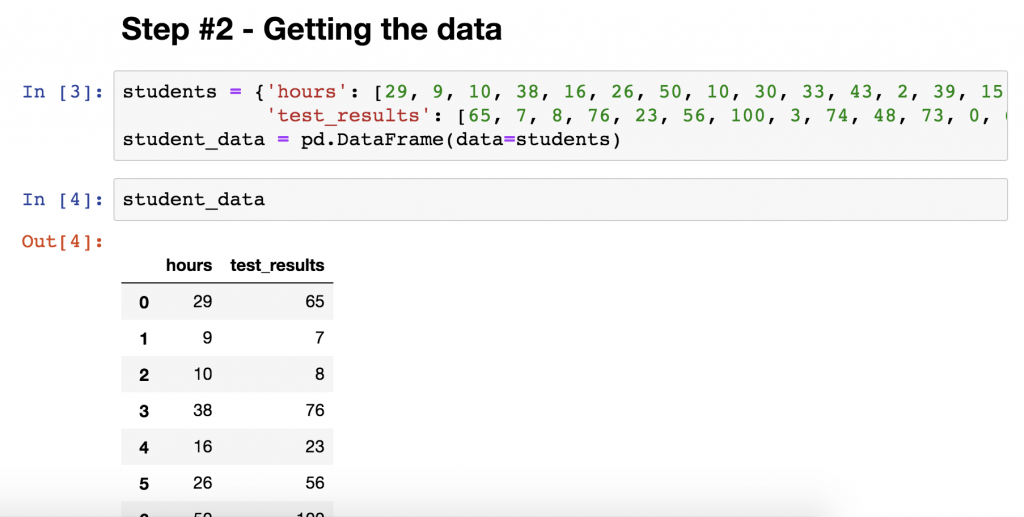
- the
hourscolumn shows how many hours each student studied - and the
test_resultscolumn shows what their test results were
(So one line is one student.)
Of course, in real life projects, we instead open .csv files (with the read_csv function) or SQL tables (with read_sql)… Regardless, the final format of the cleaned and prepared data will be a similar dataframe.
So this is your data, you will fine-tune it and make it ready for the machine learning step.
Note: And another thought about real life machine learning projects… In this tutorial, we are working with a clean dataset. That’s quite uncommon in real life data science projects. A big part of the data scientist’s job is data cleaning and data wrangling: like filling in missing values, removing duplicates, fixing typos, fixing incorrect character coding, etc. Just so you know.
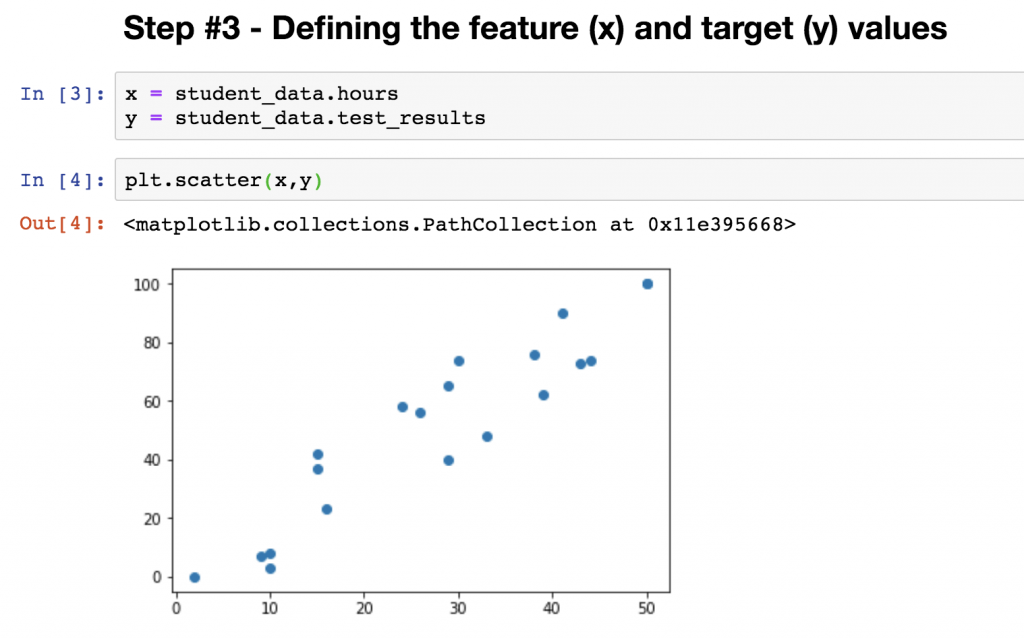
STEP #3 – Defining the feature and target values
Okay, so we have the data set.
But we have to tweak it a bit — so it can be processed by numpy‘s linear regression function.
The next required step is to break the dataframe into:
- input (x) values: this will be the
hourscolumn - and output (y) values: and this is the
test_resultscolumn
polyfit requires you to define your input and output variables in 1-dimensional format. For that, you can use pandas Series.
Let’s type this into the next cell of your Jupyter notebook:
x = student_data.hours
y = student_data.test_results
Okay, the input and output — or, using their fancy machine learning names, the feature and target — values are defined.
At this step, we can even put them onto a scatter plot, to visually understand our dataset.
It’s only one extra line of code:
plt.scatter(x,y)
And I want you to realize one more thing here: so far, we have done zero machine learning… This was only old-fashioned data preparation.
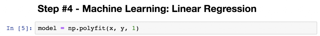
STEP #4 – Machine Learning: Linear Regression (line fitting)
We have the x and y values… So we can fit a line to them!
The process itself is pretty easy.
Type this one line:
model = np.polyfit(x, y, 1)
This executes the polyfit method from the numpy library that we have imported before. It needs three parameters: the previously defined input and output variables (x, y) — and an integer, too: 1. This latter number defines the degree of the polynomial you want to fit.
Using polyfit, you can fit second, third, etc… degree polynomials to your dataset, too. (That’s not called linear regression anymore — but polynomial regression. Anyway, more about this in a later article…)
But for now, let’s stick with linear regression and linear models – which will be a first degree polynomial. So you should just put: 1.
When you hit enter, Python calculates every parameter of your linear regression model and stores it into the model variable.
This is it, you are done with the machine learning step!
Note: isn’t it fascinating all the hype there is around machine learning — especially now that it turns that it’s less than 10% of your code? (In real life projects, it’s more like less than 1%.) The real (data) science in machine learning is really what comes before it (data preparation, data cleaning) and what comes after it (interpreting, testing, validating and fine-tuning the model).
STEP #4 side-note: What’s the math behind the line fitting?
Now, of course, fitting the model was only one line of code — but I want you to see what’s under the hood. How did polyfit fit that line?
It used the ordinary least squares method (which is often referred to with its short form: OLS). It is one of the most commonly used estimation methods for linear regression. There are a few more. But the ordinary least squares method is easy to understand and also good enough in 99% of cases.
Let’s see how OLS works!
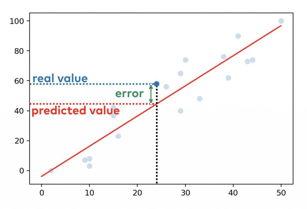
When you fit a line to your dataset, for most x values there is a difference between the y value that your model estimates — and the real y value that you have in your dataset. In machine learning, this difference is called error.
Let’s see an example!
Here’s a visual of our dataset (blue dots) and the linear regression model (red line) that you have just created. (I’ll show you soon how to plot this graph in Python — but let’s focus on OLS for now.)
Let’s take a data point from our dataset.
x = 24
In the original dataset, the y value for this datapoint was y = 58. But when you fit a simple linear regression model, the model itself estimates only y = 44.3. The difference between the two is the error for this specific data point.
So the ordinary least squares method has these 4 steps:
1) Let’s calculate all the errors between all data points and the model.
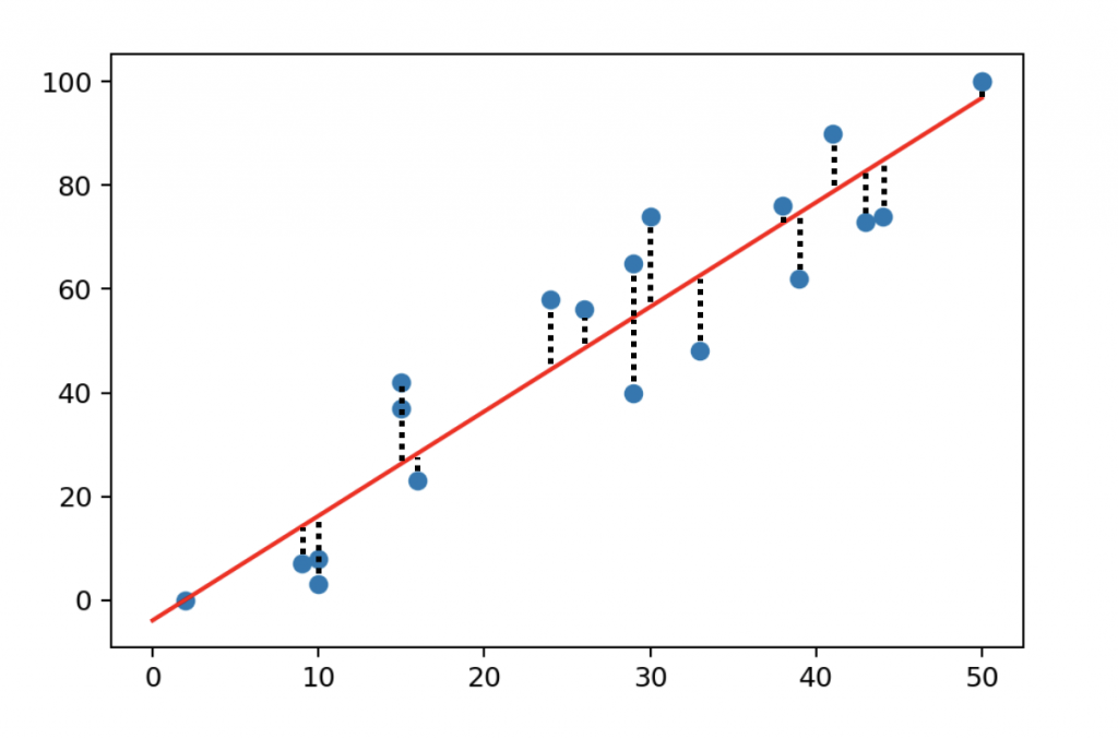
2) Let’s square each of these error values!
3) Then sum all these squared values!
4) Find the line where this sum of the squared errors is the smallest possible value.
That’s OLS and that’s how line fitting works in numpy polyfit‘s linear regression solution.
STEP #5 – Interpreting the results
Okay, so you’re done with the machine learning part. Let’s see what you got!
First, you can query the regression coefficient and intercept values for your model. You just have to type:
model
Note: Remember, model is a variable that we used at STEP #4 to store the output of np.polyfit(x, y, 1).
The output is:
array([ 2.01467487, -3.9057602 ])
These are the a and b values we were looking for in the linear function formula.
2.01467487 is the regression coefficient (the a value) and -3.9057602 is the intercept (the b value).
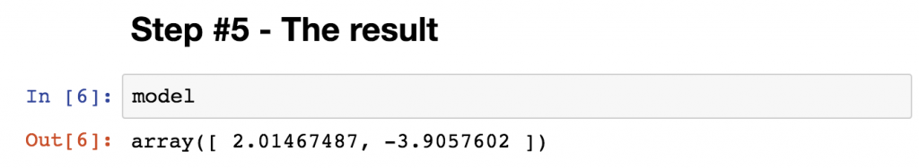
So we finally got our equation that describes the fitted line. It is:
y = 2.01467487 * x - 3.9057602
If a student tells you how many hours she studied, you can predict the estimated results of her exam. Quite awesome!
You can do the calculation “manually” using the equation.
But there is a simple keyword for it in numpy — it’s called poly1d():
predict = np.poly1d(model)
hours_studied = 20
predict(hours_studied)
The result is: 36.38773723
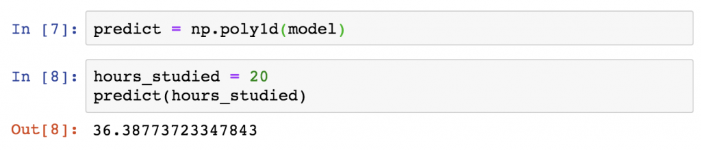
Note: This is the exact same result that you’d have gotten if you put the hours_studied value in the place of the x in the y = 2.01467487 * x - 3.9057602 equation.
So from this point on, you can use these coefficient and intercept values – and the poly1d() method – to estimate unknown values.
And this is how you do predictions by using machine learning and simple linear regression in Python.
Well, okay, one more thing…
There are a few methods to calculate the accuracy of your model. In this article, I’ll show you only one: the R-squared (R2) value. I won’t go into the math here (this article has gotten pretty long already)… it’s enough if you know that the R-squared value is a number between 0 and 1. And the closer it is to 1 the more accurate your linear regression model is.
Unfortunately, R-squared calculation is not implemented in numpy… so that one should be borrowed from sklearn (so we can’t completely ignore Scikit-learn after all :-)):
from sklearn.metrics import r2_score
r2_score(y, predict(x))
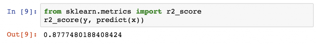
And now we know our R-squared value is 0.877.
That’s pretty nice!
STEP #6 – Plotting the linear regression model
Visualization is an optional step but I like it because it always helps to understand the relationship between our model and our actual data.
Thanks to the fact that numpy and polyfit can handle 1-dimensional objects, too, this won’t be too difficult.
Type this into the next cell of your Jupyter Notebook:
x_lin_reg = range(0, 51)
y_lin_reg = predict(x_lin_reg)
plt.scatter(x, y)
plt.plot(x_lin_reg, y_lin_reg, c = 'r')
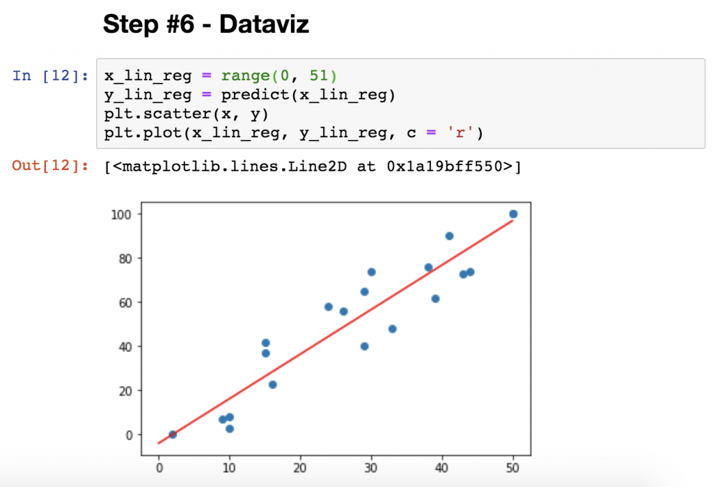
Here’s a quick explanation:
x_lin_reg = range(0, 51)
This sets the range you want to display the linear regression model over — in our case it’s between 0 and 50 hours.y_lin_reg = predict(x_lin_reg)This calculates theyvalues for all thexvalues between0and50.plt.scatter(x, y)This plots your original dataset on a scatter plot. (The blue dots.)plt.plot(x_lin_reg, y_lin_reg, c = 'r')
And this line eventually prints the linear regression model — based on thex_lin_regandy_lin_regvalues that we set in the previous two lines. (c = 'r'means that the color of the line will be red.)
Nice, you are done: this is how you create linear regression in Python using numpy and polyfit.
This was only your first step toward machine learning
You are done with building a linear regression model!
But this was only the first step. In fact, this was only simple linear regression. But there is multiple linear regression (where you can have multiple input variables), there is polynomial regression (where you can fit higher degree polynomials) and many many more regression models that you should learn. Not to speak of the different classification models, clustering methods and so on…
Here, I haven’t covered the validation of a machine learning model (e.g. when you break your dataset into a training set and a test set), either. But I’m planning to write a separate tutorial about that, too.
Anyway, I’ll get back to all these, here, on the blog!
So stay tuned!
Conclusion
Linear regression is the most basic machine learning model that you should learn.
If you understand every small bit of it, it’ll help you to build the rest of your machine learning knowledge on a solid foundation.
Knowing how to use linear regression in Python is especially important — since that’s the language that you’ll probably have to use in a real life data science project, too.
This article was only your first step! So stay with me and join the Data36 Inner Circle (it’s free).
- If you want to learn more about how to become a data scientist, take my 50-minute video course: How to Become a Data Scientist. (It’s free!)
- Also check out my 6-week online course: The Junior Data Scientist’s First Month video course.
Cheers,
Tomi Mester
Cheers,
Tomi Mester