K-means Clustering with scikit-learn (in Python)

You’re here for two reasons: 1) you want to learn to create a K-means clustering model in Python, and 2) you’re a cool person because of that (people reading data36.com are cool persons 😎).

Back to reason number one: it’s not surprising, because K-means clustering is one of the most popular and easy-to-grasp unsupervised machine learning models.

Lucky for you, you’re about to learn everything you need to know to get your feet wet. To code along with me, you have to have these libraries installed: pandas, scikit-learn, matplotlib.

Also, some basic knowledge of Python, statistics, and machine learning won’t hurt, either.

Let the fun begin. 😉

The difference between supervised and unsupervised machine learning, and why the latter can be scary

Broadly speaking, machine learning models can be categorized as either supervised or unsupervised.

Supervised means that your model receives both the “questions” (input data) and the “answers” (output data) during learning. So if you want your model to recognize whales, you can show images of different animals (input data) to it and also the solutions (output data, e.g. “this image shows a whale”, but “this image shows a lion, so it’s not a whale”).

This is a classification problem; however, supervised algorithms can be used to solve regression tasks as well (e.g. predicting the price of a car based on its attributes). If you’d like to learn more about these topics, you can find relevant articles on data36 for both types of supervised models (regression, classification).

With unsupervised learning, the story is a bit different. You don’t have any answers that supervise the model’s learning, just the inputs. You basically tell the model to do whatever it wants to do with the data.

And it’s kind of cool because unsupervised models can find hidden patterns and relationships in your dataset that you’d otherwise never be able to find (not even in your lifetime).

You don’t know what aspects of the data points the model takes into consideration when drawing its conclusions, but you don’t even care, because you just want to see what your model figured out on its own. An example would be finding different groups of this blog’s visitors based on what articles they read. Well, actually, we have created an analysis like that before:

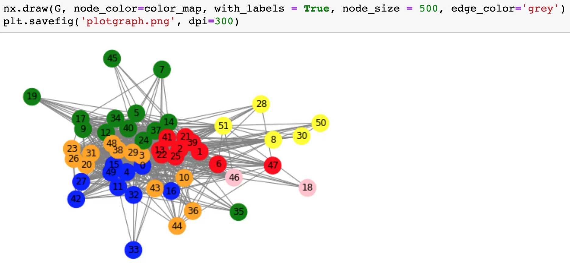
To perform such a task, you need to use something called clustering.

Note: don’t worry about what exactly you see in the picture above. It’s just a random example of clustering. But before anything else, you have to understand what clustering is in machine learning.

What is clustering in machine learning?

Clustering means grouping.

*crickets chirping*

No, seriously. 🙂 Just remember – in the context of unsupervised learning, we let our model take control, and make its own decisions. In the case of clustering, the model studies the dataset to find similarities and differences between the data points, then it creates distinct groups out of those data points.

Here’s the funny (scary?) part: once the model is done with clustering, we are left on our own.

What do I mean by that?

The model creates the groups, but it won’t attach an explanation to them detailing what each group is about, and why certain data points belong to one group and not the other. It won’t say “this group contains people who tend to spend more money on Sundays” or “this group contains cars that will break down in 5 years”.

The model will only say that this data point belongs to group a, and that belongs to group b – interpreting the clusters will be totally up to you.

Let’s see how K-means clustering – one of the most popular clustering methods – works.

Here’s how K-means clustering does its thing

You’ll love this because it’s just a few simple steps! 🤗

For starters, let’s break down what K-means clustering means:

• clustering: the model groups data points into different clusters,
• K: K is a variable that we set; it represents how many clusters we want our model to create,
• means: each cluster has a mean, and each data point will be assigned to the cluster whose mean is closest to the given data point. Read on, and you’ll get it, I promise!

Let’s look at an example. We have the following data points that we’d like to group into three groups (K = 3):

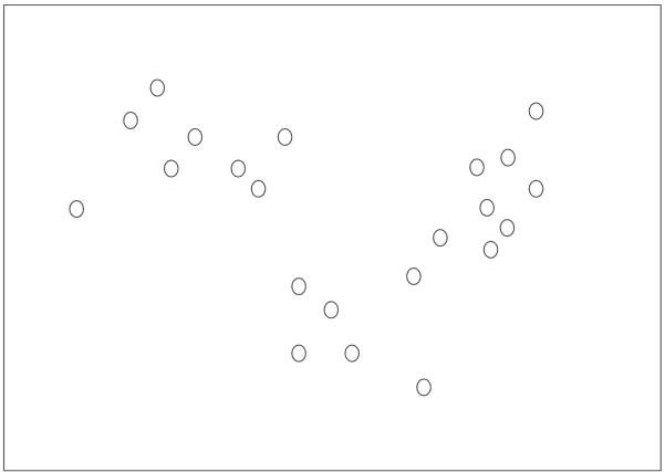
Here’s how our K-means clustering model goes about it.

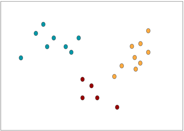
First, it randomly selects three data points (I’ve marked them with different colors):

These points are called cluster centroids because they mark the center of the clusters.

Our model then measures – using Euclidean distance – the distance of each data point to the cluster centroids, and assigns each data point to the cluster whose centroid is closest to the data point:

Now that we have three groups, each group’s cluster centroid gets recalculated (=will move to a new position) based on the average of the data points within the group, then the data points get assigned again to the closest cluster centroid (marked with a cross). Notice how data points can switch teams:

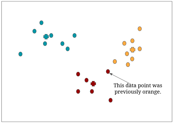
The algorithm repeats the above steps until the data points stop switching groups (=each data point is assigned to its final group, no more team switching for them).

And that’s it. 🙂

I believe two questions arise at this point:

1. Is that all? Answer: yep.
2. How do we know what value to choose for K? Answer: you’ll find it out in the coding section. 😉

How can you code a K-means clustering model in Python

I. Dropping unnecessary rows/columns before clustering

We’ll work with a dataset from Kaggle (download it from here).

The dataset contains customer data, like gender, age, profession, size of family, etc. Our plan is to create clusters out of these customers.

Read in the dataset, save it to df, and view five random rows of it with the sample method:

df = pd.read_csv("file-location-don't-copy/Train.csv")
df.sample(5, random_state=44)

Here’s the output:

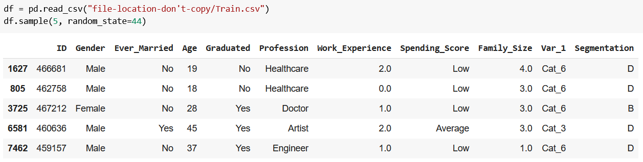
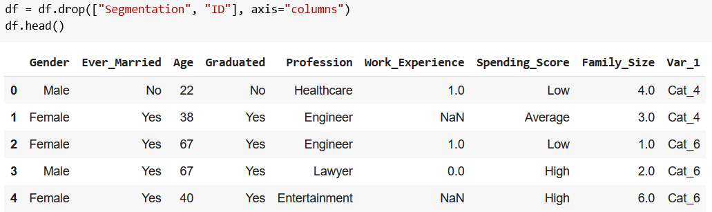
As the Segmentation column suggests, the customers have been already segmented by a certain logic (if you read the dataset’s description, you’ll know the full story). Since we want to create our own clusters, let’s remove this column along with ID:

df = df.drop(["Segmentation", “ID”], axis="columns")

A quick df.head() will attest to our success:

It’s always recommended to get a general sense of the dataset you’re working with, so let’s do just that with df.info():

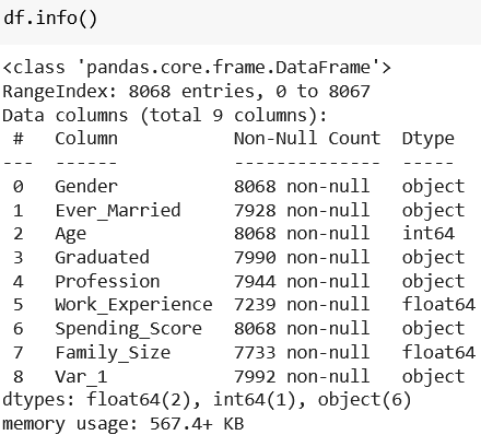
According to the RageIndex part, our dataframe (df) holds 8,068 rows. By looking at the number of data points in each column, we can establish that we have many missing data points (e.g. Graduated has 7,990 rows instead of 8,068).

For the sake of simplicity, we remove all rows with any missing values with df.dropna():

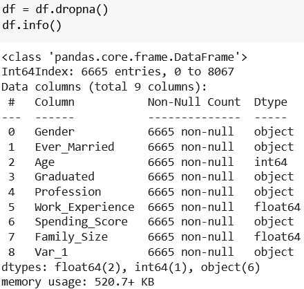
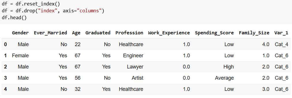
df.info() now shows that all columns have 6,665 rows, but our index still goes from 0 to 8067, so we reset it with df.reset_index(), then remove the freshly created index column with df.drop("index", axis="columns"):

df = df.reset_index()
df = df.drop("index", axis="columns")
df.head()

Perfection:

I’ll level with you: to create a K-means clustering model, it’d be perfectly fine if you just removed the Segmentation and the ID columns, and the rows with missing values.

But I like to keep my data neat and organized, so that’s why you had to go through all this – sorry!

I’ll make it up to you by showing you the fun part, okay? 🙂

II. Formatting the data for the K-means clustering model

Since our soon-to-be existing model doesn’t understand categorical data (e.g. Graduated = No), we need to convert categorical values to numerical data:

df_new = pd.get_dummies(df)
df_new.head()

The output:

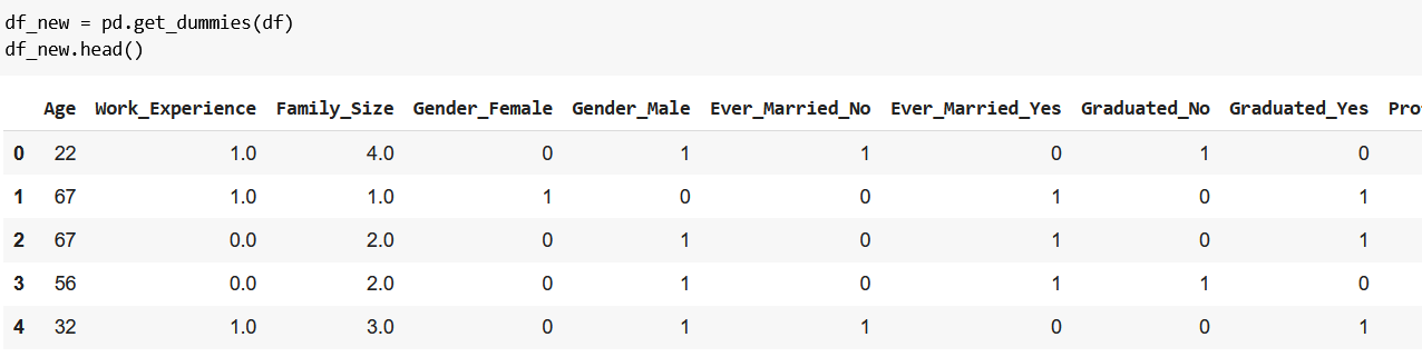
pd.get_dummies() successfully converted our data, and that we’re happy about! 🙂 What we’re not happy about is the many rows that don’t even fit in one screenshot. 😟

Before we fix that, let me explain what just happened:

• previously we had columns holding categorical data (e.g. Graduated = No),
• after get_dummies(), we have numerical columns representing our categorical data (e.g. Graduated_No = 1 or 0),
• where 1 means true and 0 means false (e.g. Graduated_No = 0 is just Graduated = No in a new form that our model understands).

If you pay close attention, you may notice that now we have plenty of redundant data: Graduated_No = 0 and Graduated_Yes = 1 both represent the same thing (that someone graduated), so we don’t need both columns. We can keep only the first of the two by adding drop_first=True to get_dummies():

df_kmeans = pd.get_dummies(df, drop_first=True)
df_kmeans.head()

The result:

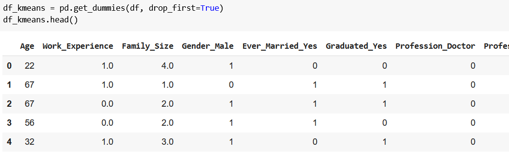
(Okay, it’s not a must step, because our model would do just fine without it, but again, I like to keep things simple – mea maxima culpa. You can check with df_new.columns.size and df_kmeans.columns.size that we managed to reduce the number of columns from 28 to 22.)

III. Standardization

Now, because we have columns with different ranges of numbers (e.g. most of them are either 0 or 1, but Age can be more than 1), we need to standardize our data. According to scikit-learn’s documentation:

“Standardization of a dataset is a common requirement for many machine learning estimators: they might behave badly if the individual features do not more or less look like standard normally distributed data […]”

Let’s just believe that, and type the following:

from sklearn.preprocessing import StandardScaler
scaler = StandardScaler()
scaled_df_kmeans = scaler.fit_transform(df_kmeans)

The first row imports StandardScaler, which does the standardization for us. The second one creates the scaler itself, and the third one actually implements it on our data (scaled_df_kmeans is the output, our standardized data).

IV. Creating the K-means clustering model!

Finally, we can create our K-means clustering model:

from sklearn.cluster import KMeans
kmeans_model = KMeans(n_clusters=3)
clusters = kmeans_model.fit_predict(df_kmeans)
df_kmeans.insert(df_kmeans.columns.get_loc("Age"), "Cluster", clusters)
df_kmeans.head(3)

I don’t want to keep you waiting, so first I show you the output, then explain what happened.

Here’s the output:

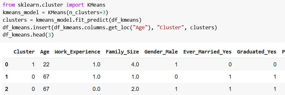
• from sklearn.cluster import KMeans imports the K-means clustering algorithm,
• KMeans(n_clusters=3) saves the algorithm into kmeans_model, where n_clusters denotes the number of clusters we’d like to create,
• kmeans_model.fit_predict(df_kmeans) clusters our customers into one of the three clusters, and then the cluster labels are saved to clusters,
• df_kmeans.insert(df_kmeans.columns.get_loc("Age"), "Cluster", clusters) creates a new column (Cluster) holding the previously created clusters’ values (aka what cluster our model assigned to each customer in our dataset); df_kmeans.columns.get_loc("Age") is responsible for inserting Cluster as the first column.

If you’re curious, df_kmeans.Cluster.unique() will show you the labels for the clusters:

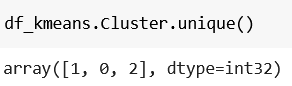
And that’s how you create a K-means clustering model. 🙂

Two more important things to know:

1. Now you should get an expert, who can help you interpret what each cluster possibly can mean.
2. You may wonder if three was the best choice for K… fortunately, there’s a method called elbow to determine the optimal number of clusters for our model. Read on to learn more about it.

Finding the ideal number of clusters with the elbow method

The so-called elbow method is a common way to find the ideal number of clusters within a dataset.

It’s called elbow, because:

1. it takes the possible values of K that you choose,
   1. for example, beginning from two clusters and going up to eight clusters the values for K would be: 2, 3, 4, 5, 6, 7, 8,
2. calculates the sum of squared distances (SSD for short) for every value of K (=number of clusters),
   1. SSD is the result of calculating in each cluster, how far the data points are from the cluster centroid, then adding up the results for all clusters; think of it as something that shows the variance of your data (fun fact: as the number of clusters increase, the SSD decreases),
3. creates a line plot where the x-axis contains the values that K can take on, and the y-axis shows the SSD (=variance) for each K (=number of clusters).

Once the above steps have been carried out, our task is to identify the elbow point (=the number for K), after which there are no more sudden drops in the line plot (=SSD is not significantly reduced, so there’s no need to add more clusters).

You’ll immediately get what I’m talking about by looking at this chart:

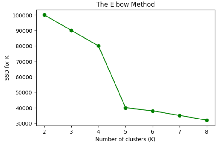
The solution here is five; after it, there seem to be no more sudden drops, so the ideal number for this dataset would be five.

We’ll apply the elbow method to our dataset with the below code:

ssd = []
for k in range(2, 9):
    kmeans_model = KMeans(n_clusters=k)
    kmeans_model.fit(df_kmeans)
    ssd.append(kmeans_model.inertia_)
plt.figure(figsize=(6, 4), dpi=100)
plt.plot(range(2, 9), ssd, color="green", marker="o")
plt.xlabel("Number of clusters (K)")
plt.ylabel("SSD for K")
plt.show()

Here’s the breakdown of the code:

• ssd is a list of the calculated SSD values for each value of K,
• we set a minimum and a maximum value for K with range(2, 9), and loop through them (for k in range(2, 9)),
• at each loop, we create a K-means clustering model for k (kmeans_model = KMeans(n_clusters=k)),
• then we fit the model (kmeans_model.fit(df_kmeans)),
• and add its calculated SSD (ssd.append(kmeans_model.inertia_)) to ssd,
  • note: inertia means SSD,
• and finally, we visualize it with the rest of the code.

Now you should see a chart like this:

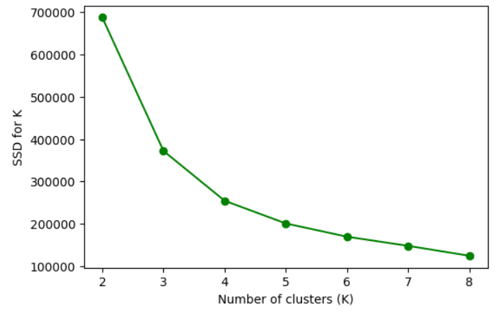
I’d say that the ideal number of clusters for this dataset is four instead of three. So we can rerun the code with K being equal to four, but I won’t do that now, because there’s still one important aspect that we need to touch on.

What if we don’t see an elbow in the chart? 🤔

Yes, it can happen. It’s not guaranteed that you’ll always get an elbow.

Why?

Because life isn’t always sunshine and puppies, and data science is hard.

But we’re tough, ain’t we? 😎

Whenever you encounter such difficulties, start googling. You’ll be encouraged by seeing others having the same problems – like here, here, or here.

The thing is, there’s always a solution. If you don’t see an elbow point, the solution could be to look at the silhouette score.

Or maybe not. 😉

Conclusion

Okay, the last sentence from the previous section may have sounded too distressing – but I didn’t mean it that way! Oftentimes, data science can be challenging, but if you take one step at a time, it can be conquered.

And you did take an important step by following this tutorial because you’ve learned about a new model. If you’re curious about other machine learning models, just click here to see what we’ve got for you.

And don’t forget – if you get stuck with a problem, just Google it! 😉

• If you want to learn more about how to become a data scientist, take Tomi Mester’s 50-minute video course: How to Become a Data Scientist. (It’s free!)
• Also check out the 6-week online course: The Junior Data Scientist’s First Month video course.

Cheers,

Tamas Ujhelyi