Polynomial Regression in Python using scikit-learn (with a practical example)

If you want to fit a curved line to your data with scikit-learn using polynomial regression, you are in the right place. But first, make sure you’re already familiar with linear regression. I’ll also assume in this article that you have matplotlib, pandas and numpy installed. Now let’s get down to coding your first polynomial regression model.

If you don’t have your own Python environment for data science, go with one of these options to get one:

• Get your own data server and install the most popular data science libraries
• Install Anaconda on your local computer

What’s polynomial regression good for? A quick example.

Bad news: you can’t just linear regression your way through every dataset. 😔

Oftentimes you’ll encounter data where the relationship between the feature(s) and the response variable can’t be best described with a straight line.

Just like here:

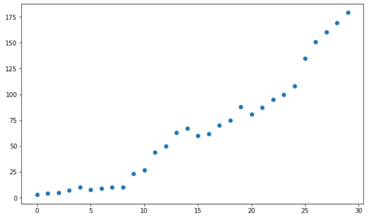
See the problem? Of course we could fit a straight line to the data, but just by looking at the scatterplot we get the feeling that this time a linear line won’t cut it.

If you think that the line should somehow be curved to better fit the data, then you intuitively understand why we use polynomial regression: it gives us the curvature we need so we can have more precise predictions based on our data.

But let’s hold our horses just yet. 🐴

Why is it called a “polynomial”?

That’s what we’ll discover in the next section.

What is a polynomial? The most important definitions you need to know.

Let’s break it down:

• “poly” means “many”,
• “nomial” means “terms” (or “parts” or “names”).

Here’s an example of a polynomial:

4x + 7

4x + 7 is a simple mathematical expression consisting of two terms: 4x (first term) and 7 (second term). In algebra, terms are separated by the logical operators + or -, so you can easily count how many terms an expression has.

9x2y - 3x + 1 is a polynomial (consisting of 3 terms), too. And to confuse you a bit, 3x is also a polynomial, although it doesn’t have “many terms” (3x is called a monomial, because it consists of one term – but don’t worry too much about it, I just wanted to let you in on this secret 🤫).

For now, let’s stick with 4x + 7. I plotted it for you:

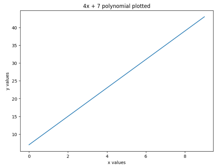
Now I want you to take a close look at the plot – what do you see? A straight line! 😮

Let’s recap what just happened:

1. we took a polynomial (4x + 7),
2. plotted it,
3. and got a straight line (remember: a linear regression model gives you a straight line).

What’s happening…? 🤔

You see, the formula that defines a straight line in a linear regression model is actually a polynomial, and it goes by its own special name: linear polynomial (anything that takes the form of ax + b is a linear polynomial).

Nice. Can we start coding already?

Actually… no.

Polynomial regression related vocabulary

Before we get to the practical part, there’s some more things you need to know.

We’ll use 3x⁴ – 7x³ + 2x² + 11 to improve your polynomial related vocabulary with some essential definitions:

• degree of a polynomial: the highest power (largest exponent) in your polynomial; in our example it’s 4 because of x4, meaning that we’re dealing with a 4^th degree polynomial,
• coefficient: each number (3, 7, 2, 11) in our polynomial is a coefficient; these are the parameters that are unknown and our polynomial regression model will try to estimate when trained on our dataset,
• leading term: the term with the highest power (in our case it’s 3x4); this is the most important part of a polynomial, because it determines the polynomial’s graph behavior,
• leading coefficient: the coefficient of the leading term (it’s 3 in our polynomial),
• constant term: the y intercept, it never changes: no matter what the value of x is, the constant term remains the same.

Polynomial Regression: the official definition

Now that you speak proper polynomial lingo, I’d like to give you an official definition. An expression is a polynomial if:

• the expression has a finite number of terms,
• and each term has a coefficient,
• and these coefficients are multiplied by a variable (in our case x),
• and the variables are raised to a non-negative integer power.

If you’ve been paying attention, you may wonder: how is 4x + 7 a polynomial when the second term (7) clearly lacks the variable x?

Actually, x is there in the form of 7xo. Since xo is equal to 1, and 7*1 is equal to 7, there’s really no need to write xo down.

The difference between linear and polynomial regression.

Let’s return to 3x4 - 7x3 + 2x2 + 11: if we write a polynomial’s terms from the highest degree term to the lowest degree term, it’s called a polynomial’s standard form.

In the context of machine learning, you’ll often see it reversed:

y = ß0 + ß1x + ß2x2 + … + ßnxn

• y is the response variable we want to predict,
• x is the feature,
• ß0 is the y intercept,
• the other ßs are the coefficients/parameters we’d like to find when we train our model on the available x and y values,
• n is the degree of the polynomial (the higher n is, the more complex curved lines you can create).

The above polynomial regression formula is very similar to the multiple linear regression formula:

y = ß0 + ß1x1 + ß2x2 + … + ßnxn

It’s not a coincidence: polynomial regression is a linear model used for describing non-linear relationships.

How is this possible? The magic lies in creating new features by raising the original features to a power.

For instance if we have feature x, and we’ll use a 3^rd degree polynomial, then our formula will also include x2 and x3. And this is what gives curvature to a line:

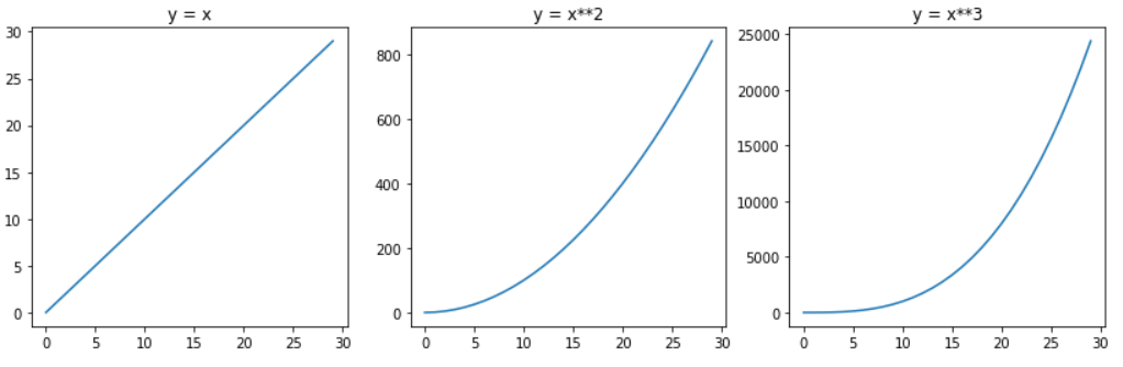
What I’m trying to hammer home is this: linear regression is just a first-degree polynomial. Polynomial regression uses higher-degree polynomials. Both of them are linear models, but the first results in a straight line, the latter gives you a curved line. That’s it.

Now you’re ready to code your first polynomial regression model.

Coding a polynomial regression model with scikit-learn

For starters, let’s imagine that you’re presented with the below scatterplot:

Here’s how you can recreate the same chart:

import numpy as np
import pandas as pd
import matplotlib.pyplot as plt

x = np.arange(0, 30)
y = [3, 4, 5, 7, 10, 8, 9, 10, 10, 23, 27, 44, 50, 63, 67, 60, 62, 70, 75, 88, 81, 87, 95, 100, 108, 135, 151, 160, 169, 179]
plt.figure(figsize=(10,6))
plt.scatter(x, y)
plt.show()

It’s nothing special, really: just one feature (x), and the responses (y).

Now, let’s say that you’ve got a hunch that the relationship between the features and the responses is non-linear, and you’d like to fit a curved line to the data.

Since we have only one feature, the following polynomial regression formula applies:

y = ß0 + ß1x + ß2x2 + … + ßnxn

In this equation the number of coefficients (ßs) is determined by the feature’s highest power (aka the degree of our polynomial; not considering ß0, because it’s the intercept).

Two questions immediately arise:

1. How do we establish the degree of our polynomial (and thus the number of ßs)?
2. How do we create x², x³ or xⁿ when originally we have x as our one and only feature?

Fortunately, there are answers to both questions.

Answer 1.: there are methods to determine the degree of the polynomial that gives the best results, but more on this later. For now, let’s just go with the assumption that our dataset can be described with a 2^nd degree polynomial.

Answer 2.: we can create the new features (x raised to increasing powers) once you’ve installed sci-kit learn.

STEP #1: Determining the degree of the polynomial

First,  import PolynomialFeatures:

from sklearn.preprocessing import PolynomialFeatures

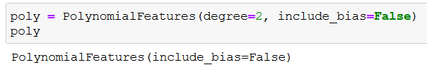
Then save an instance of PolynomialFeatures with the following settings:

poly = PolynomialFeatures(degree=2, include_bias=False)

degree sets the degree of our polynomial function. degree=2 means that we want to work with a 2^nd degree polynomial:

y = ß0 + ß1x + ß2x2

include_bias=False should be set to False, because we’ll use PolynomialFeatures together with LinearRegression() later on.

Long story short: LinearRegression() will take care of this setting by default, so there’s no need to set include_bias to True. If it wasn’t taken care of, then include_bias=False would mean that we deliberately want the y intercept (ß0) to be equal to 0 – but we don’t want that. Here’s a great explanation on all of this.

If you print poly, you see that so far we’ve just created an instance of PolynomialFeatures, and that’s all there’s to it:

Onto the next step:

STEP #2: Creating the new features

poly_features = poly.fit_transform(x.reshape(-1, 1))

reshape(-1,1) transforms our numpy array x from a 1D array to a 2D array – this is required, otherwise we’d get the following error:

There’s only one method – fit_transform() – but in fact it’s an amalgam of two separate methods: fit() and transform(). fit_transform() is a shortcut for using both at the same time, because they’re often used together.

Since I want you to understand what’s happening under the hood, I’ll show them to you separately.

With fit() we basically just declare what feature we want to transform:

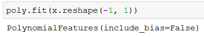
transform() performs the actual transformation:

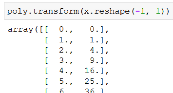
What are these numbers? Well, let me kindly remind you that our feature values in the scatterplot range from 0 to 29. In the first column we have our values for x (e.g. 3). In the second column we have our values for x squared (e.g. 9).

Looks familiar? Our 2^nd degree polynomial formula, again:

y = ß0 + ß1x + ß2x2

We wanted to create x² values from our x values, and fit_transform() did just that. We save the result to poly_features:

poly_features = poly.fit_transform(x.reshape(-1, 1))

STEP #3: Creating the polynomial regression model

Now it’s time to create our machine learning model. Of course, we need to import it first:

from sklearn.linear_model import LinearRegression

Hold up a minute! 😮 Isn’t this tutorial supposed to be about polynomial regression? Why are we importing LinearRegression then?

Just think back to what you’ve read not so long ago: polynomial regression is a linear model, that’s why we import LinearRegression. 🙂

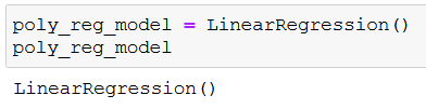
Let’s save an instance of LinearRegression to a variable:

poly_reg_model = LinearRegression()

Here’s the code in real life:

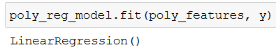
Then we fit our model to our data:

poly_reg_model.fit(poly_features, y)

Fitting means that we train our model by letting it know what the feature (poly_features) and the response (y) values are. When fitting/training our model, we basically instruct it to solve for the coefficients (marked with bold) in our polynomial function:

y = ß0 + ß1x + ß2x2

After running the code you may think that nothing happens, but believe me, the model estimated the coefficients (important: you don’t have to save it to a variable in order for it to work!):

Now that our model is properly trained, we can put it to work by instructing it to predict the responses (y_predicted) based on poly_features, and the coefficients it had estimated:

y_predicted = poly_reg_model.predict(poly_features)

Here you can see the predicted responses:

Let’s do some dataviz to see what our model looks like:

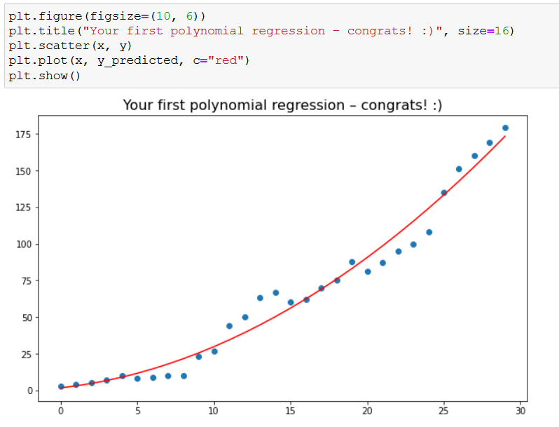
I think the plot’s title says it all, but I’d like to repeat it: congratulations, you’ve created your very first polynomial regression model! 👏

While you’re celebrating, I’m just gonna paste the code here in case you need it:

plt.figure(figsize=(10, 6))
plt.title("Your first polynomial regression – congrats! :)", size=16)
plt.scatter(x, y)
plt.plot(x, y_predicted, c="red")
plt.show()

Coding a polynomial regression model with multiple features

Oftentimes you’ll have to work with data that includes more than one feature (life is complicated, I know). Let’s simulate such a situation:

import numpy as np
import pandas as pd
import matplotlib.pyplot as plt

np.random.seed(1)
x_1 = np.absolute(np.random.randn(100, 1) * 10)
x_2 = np.absolute(np.random.randn(100, 1) * 30)
y = 2*x_1**2 + 3*x_1 + 2 + np.random.randn(100, 1)*20

np.random.seed(1) is needed so you and I can work with the same “random” data. (Read this article if you want to understand how it is possible.) We create some random data with some added noise: x_1 contains 100 values for our first feature, x_2 holds 100 values for our second feature. Our responses (100) are saved into y, as always.

Let’s plot both features, just to get a visualized understanding of the relationships between the features and the responses:

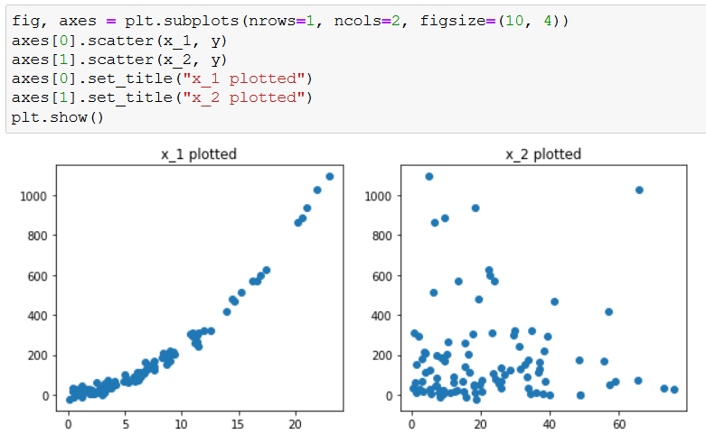
For your convenience, here’s the code:

fig, axes = plt.subplots(nrows=1, ncols=2, figsize=(10, 4))
axes[0].scatter(x_1, y)
axes[1].scatter(x_2, y)
axes[0].set_title("x_1 plotted")
axes[1].set_title("x_2 plotted")
plt.show()

STEP #1: Storing the variables in a dataframe

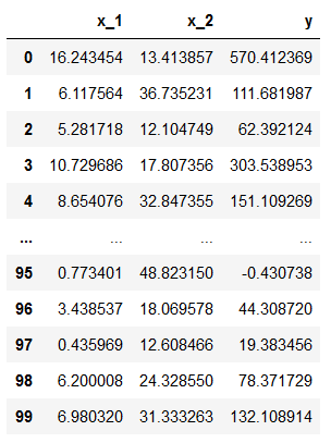
Then we create a pandas dataframe where we’ll store our features and responses:

df = pd.DataFrame({"x_1":x_1.reshape(100,), "x_2":x_2.reshape(100,), "y":y.reshape(100,)}, index=range(0,100))
df

This is the resulting dataframe:

Again, reshape(100,) is needed (100, because we have 100 rows), otherwise we’d receive the following error:

STEP #2: Defining the training and the test data

Now we turn to scikit-learn again:

from sklearn.model_selection import train_test_split

train_test_split helps us split our data into a training and a test dataset:

X, y = df[["x_1", "x_2"]], df["y"]
poly = PolynomialFeatures(degree=2, include_bias=False)
poly_features = poly.fit_transform(X)
X_train, X_test, y_train, y_test = train_test_split(poly_features, y, test_size=0.3, random_state=42)

Here’s a step by step explanation:

1. X, y = df[["x_1", "x_2"]], df["y"]: From df, we save the x_1 and x_2 columns to X, the y column to y. At this point we have the features and the responses stored in separate variables.
2. poly = PolynomialFeatures(degree=2, include_bias=False) and poly_features = poly.fit_transform(X): just as before, we create the new polynomial features.
3. train_test_split(poly_features, y, test_size=0.3, random_state=42): Within the train_test_split method we define all of our features (poly_features) and all of our responses (y). Then, with test_size we set what percentage of our all features (poly_features) and responses (y) we’d like to allocate for testing our model’s prediction capability. In our case, it’ll be 30% (0.3), because it’s a good practice. Don’t worry if it’s not clear at first: you’ll understand it in a minute.  random_state needs to receive an integer value: that way anytime you rerun train_test_split, you’ll receive the same results.
4. X_train, X_test, y_train, y_test: train_test_split splits our features (poly_features) and responses (y) into train and test groups – here we just save these groups into variables. The order of the variables is very important, so don’t shuffle them.

STEP #3: Creating a polynomial regression model

Now let’s create and fit our model, but this time, we’ll train our model only on the training data:

poly_reg_model = LinearRegression()
poly_reg_model.fit(X_train, y_train)

The reason for us training our model only on the training data is that later we want to see how well our model will predict responses based on feature values it hasn’t seen before.

Here’s how we can test how our model performs on previously unseen data:

poly_reg_y_predicted = poly_reg_model.predict(X_test)
from sklearn.metrics import mean_squared_error
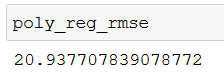
poly_reg_rmse = np.sqrt(mean_squared_error(y_test, poly_reg_y_predicted))
poly_reg_rmse

It may be a lot to take in, so let me elaborate on it:

• poly_reg_y_predicted = poly_reg_model.predict(X_test): We save the predicted values our model predicts based on the previously unseen feature values (X_test).
• from sklearn.metrics import mean_squared_error: We import mean_squared_error – more on why in the next bullet point.
• poly_reg_rmse = np.sqrt(mean_squared_error(y_test, poly_reg_y_predicted)): We take the square root of mean_squared_error to get the RMSE (root mean square error) which is a commonly used metric to evaluate a machine learning model’s performance. RMSE shows how far the values your model predicts (poly_reg_y_predicted) are from the true values (y_test), on average. Roughly speaking: the smaller the RMSE, the better the model.

If you print poly_reg_rmse, you’ll get this number:

STEP #4: Creating a linear regression model

Now let’s create a linear regression model as well, so we can compare the performance of the two models:

X_train, X_test, y_train, y_test = train_test_split(X, y, test_size=0.3, random_state=42)
lin_reg_model = LinearRegression()
lin_reg_model.fit(X_train, y_train)
lin_reg_y_predicted = lin_reg_model.predict(X_test)
lin_reg_rmse = np.sqrt(mean_squared_error(y_test, lin_reg_y_predicted))
lin_reg_rmse

As you can see, the steps are the same as in the case of our polynomial regression model. There’s one important difference, though. In the train_test_split method we use X instead of poly_features, and it’s for a good reason. X contains our two original features (x_1 and x_2), so our linear regression model takes the form of:

y = ß0 + ß1x1 + ß2x2

If you print lin_reg_model.coef_ you can see the linear regression model’s values for ß1 and ß2:

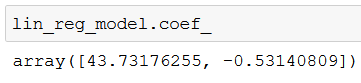
You can similarly print the intercept with lin_reg_model.intercept_:

On the other hand, poly_features contains new features as well, created out of x_1 and x_2, so our polynomial regression model (based on a 2^nd degree polynomial with two features) looks like this:

y = ß0 + ß1x1 + ß2x2 + ß3x12 + ß4x22 + ß5x1x2

This is because poly.fit_transform(X) added three new features to the original two (x₁ (x_1) and x₂ (x_2)): x₁², x₂² and x₁x₂.

x₁² and x₂² need no explanation, as we’ve already covered how they are created in the “Coding a polynomial regression model with scikit-learn” section.

What’s more interesting is x₁x₂ – when two features are multiplied by each other, it’s called an interaction term. An interaction term accounts for the fact that one variable’s value may depend on another variable’s value (more on this here). poly.fit_transform() automatically created this interaction term for us, isn’t that cool? 🙂

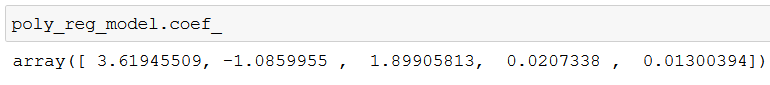
Accordingly, if we print poly_reg_model.coef_, we’ll get the values for five coefficients (ß1, ß2, ß3, ß4, ß5):

But let’s get back to comparing our models’ performances by printing lin_reg_rmse:

The RMSE for the polynomial regression model is 20.94 (rounded), while the RMSE for the linear regression model is 62.3 (rounded). The polynomial regression model performs almost 3 times better than the linear regression model. That’s a spectacular difference.

But you know what else is spectacular?

Your freshly gained knowledge on performing polynomial regression! 😉

Conclusion

Hopefully you’ve gained enough knowledge to have a basic understanding of polynomial regression. Not only that, you should also know one method (RMSE) for comparing the performance of machine learning models.

Throughout this article we used a 2^nd degree polynomial for our polynomial regression models. Naturally, you should always test before model deployment what degree of polynomial performs best on your dataset (after finishing this article, you should suspect how to do that! 😉).

Thank you for reading this article, and have fun with your new knowledge!

• If you want to learn more about how to become a data scientist, take Tomi Mester’s 50-minute video course: How to Become a Data Scientist. (It’s free!)
• Also check out the 6-week online course: The Junior Data Scientist’s First Month video course.

Cheers,

Tamas Ujhelyi