Random Forest in Python (and coding it with Scikit-learn)

If you already know how to code decision trees, it’s only natural that you want to go further – why stop at one tree when you can have many? Good news for you: the concept behind random forest in Python is easy to grasp, and they’re easy to implement.

In this tutorial, you’ll learn what random forests are and how to code one with scikit-learn in Python. For reading this article, knowing about regression and classification decision trees is considered to be a prerequisite. Also, having matplotlib, pandas and scikit-learn installed is required for the full experience. 🙂

Note: this article can help to setup your data server and then this one to install data science libraries.

I’d like to point out that we’ll code a random forest for a classification task. The reason for this is simple: in a real-life situation, I believe it’s more likely that you’ll have to solve a classification task rather than a regression task.

With that in mind, let’s first understand what a random forest is and why it’s better than a simple decision tree.

Random Forest – what is it?

I. A random forest is a bunch of different decision trees that overcome overfitting

That’s what the forest part means; if you put together a bunch of trees, you get a forest. Big brain time, right? 🙂

In all seriousness, there’s a very clever motive behind creating forests. If you recall, decision trees are not the best machine learning algorithms, partly because they’re prone to overfitting.

Why?

A decision tree trained on a certain dataset is defined by its settings (e.g. depth, splitting criterion, etc.). If you create a model with the same settings for the same dataset, you’ll get the exact same decision tree (same root node, same splits, same everything).

And if you introduce new data to your decision tree… oh boy, overfitting happens! 😐

Problem is, we really don’t want overfitting to happen, so somehow we need to create different trees. Different trees mean that each tree offers a unique perspective on our data (=they have different settings). We want this because these unique perspectives lead to an improved, collective understanding of our dataset.

Long story short, this collective wisdom is achieved by creating many different decision trees. This is also what reduces overfitting and generates better predictions compared to that of a single decision tree.

The million-dollar question, then, is this: how do we get different trees?

And this is the exciting part. The random part.

II. A random forest is random because we randomize the features and the input data for its decision trees

II/I. Randomizing the features

You already know that a decision tree doesn’t always use all of the features of a dataset. This is not necessarily okay, because omitted features can still be important in understanding your dataset.

So what does a random forest do?

At each split of a decision tree, it randomizes the features that it takes into consideration. By doing this, it gives a chance to every feature in the dataset to have its say in classifying data.

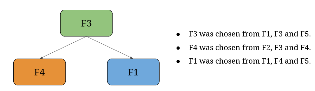
Let me explain with a quick example. If you have a dataframe with five features (F1, F2, F3, F4, and F5), at every split in a decision tree a certain number (let’s settle for three for now) of features will be randomly chosen, and the split will be carried out based on one of these features.

As a result, one of your decision trees might look like this (with more splits, of course):

But another one could look like this (naturally, with more splits):

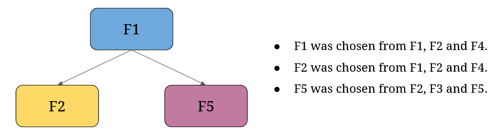
And this happens to each decision tree in a random forest model. You can already see why this method results in different decision trees.

But this is only one side of the coin; let’s check out the other.

II/II. Bootstrapping: Randomizing the input data

For each decision tree, a new dataset is formed out of the original dataset. These newly formed datasets have the exact same number of rows as the original dataset. The rows are picked with random sampling with replacement, meaning that the exact same row can be contained in the new dataset more than once.

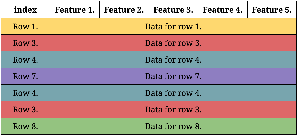
This process is called bootstrapping. Let’s illustrate this with an example where your dataset has 8 rows from 1 to 8. A bootstrapped dataset can include a row more than once, so your bootstrapped dataset could look like this:

Randomizing the features at each split, together with bootstrapping, creates different decision trees. These two randomization processes are at the heart of random forests; they are responsible for eliminating the overfitting issues of decision trees.

Now we know how different decision trees are created in a random forest. What’s left for us is to gain an understanding of how random forests classify data.

Bagging: the way a random forest produces its output

So far we’ve established that a random forest comprises many different decision trees with unique opinions about a dataset. If opinions differ, how will a random forest come to a final decision?

Meet bagging.

Bagging means bootstrap aggregating or bootstrap aggregation.

The bootstrap part you already know and understand. What is aggregation, then?

You see, in a random forest there are many decision trees that are trained on bootstrapped data – if you give input to each decision tree, each decision tree will give you a prediction to the best of its tree-specific knowledge (=based on the bootstrapped data it’s been fitted on).

Aggregation means that each tree has its own vote, then the votes are counted, and the prediction with the most votes will be announced as the winner (=the output of your random forest model).

Let’s say you want to predict whether an animal is a tiger or a zebra. You create a random forest with 1000 decision trees in it, you train the trees on bootstrapped data, then give them new input data based on which they have to decide if the animal is a tiger or a zebra.

The result is the following: out of the 1000 decision trees 940 vote for the animal to be a zebra, while 60 of them say it’s a tiger. Based on all of the votes, you can be pretty sure that the animal in question is a zebra.

How sure can you be exactly?

That’s one of the beauties of random forests – you not only get a prediction, but also a probability accompanied by it. 940 is 94% of 1000, so you can be 94% sure that your model’s prediction is correct.

That’s all you need to know for now. If you’re interested in bagging in more detail, I highly recommend you watch this lecture by Kilian Weinberger.

Random Forest in Python (coding it with scikit-learn step-by-step)

Step 1. – Separating the features and the label

For starters, don’t forget to import pandas:

import pandas as pd

Then download the dataset – we’ll use the same Possum Regression dataset from the regression tree tutorial to predict a possum’s sex based on its characteristics like belly size, skull width, etc.

As stated on the dataset’s page:

“Data originally found in the DAAG R package and used in the book Maindonald, J.H. and Braun, W.J. (2003, 2007, 2010) “Data Analysis and Graphics Using R”).

A subset of the data was also put together for the OpenIntro Statistics book chapter 8 Introduction to linear regression.

Original Source of dataset:

Lindenmayer, D. B., Viggers, K. L., Cunningham, R. B., and Donnelly, C. F. 1995. Morphological variation among columns of the mountain brushtail possum, Trichosurus caninus Ogilby (Phalangeridae: Marsupialia). Australian Journal of Zoology 43: 449-458.”

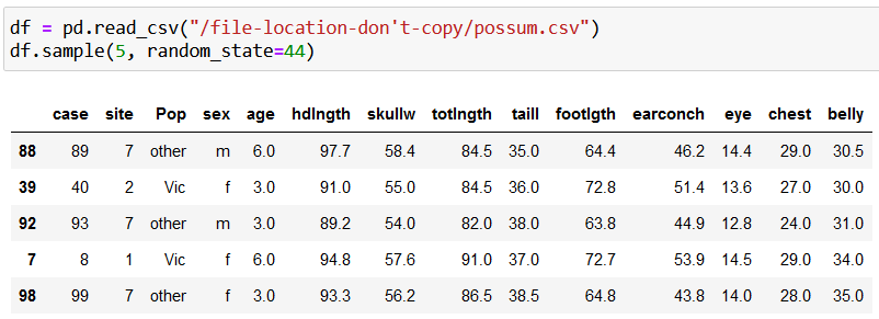
Next, read the data in, and investigate five rows from it at random with:

df = pd.read_csv("/file-location-don't-copy/possum.csv")
df.sample(5, random_state=44)

Here’s the result:

Let’s do a quick clean up and remove any rows with missing data with:

df = df.dropna()

(If you do df.info() before and after df.dropna(), you’ll see that we’ve removed three rows from the dataframe.)

Now let’s remove the unnecessary columns, then store the features and the label data in separate variables:

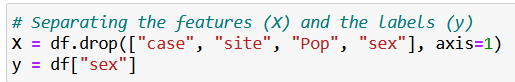
Here’s the code in case you’d like to copy it:

X = df.drop(["case", "site", "Pop", "sex"], axis=1)
y = df["sex"]

Step 2. – Training our random forest model

At this step we’ll create our first random forest:

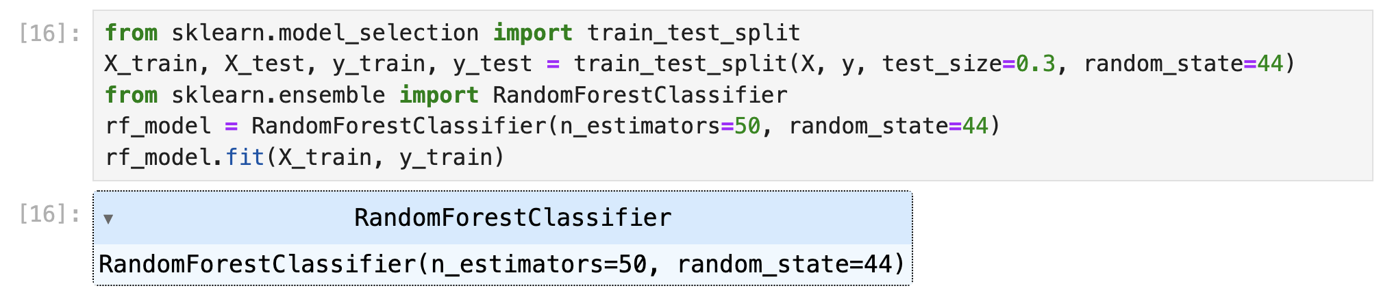
from sklearn.model_selection import train_test_split
X_train, X_test, y_train, y_test = train_test_split(X, y, test_size=0.3, random_state=44)
from sklearn.ensemble import RandomForestClassifier
rf_model = RandomForestClassifier(n_estimators=50, random_state=44)
rf_model.fit(X_train, y_train)

Let me break the above code down for you (although I think it’s already familiar to you at this point if you’ve read the previous articles on machine learning models):

• from sklearn.model_selection import train_test_split >> This line imports train_test_split which we’ll make it possible to randomly separate our dataset into train and test data.
• X_train, X_test, y_train, y_test = train_test_split(X, y, test_size=0.3, random_state=44) >> This is where we allocate 30% (test_size=0.3) of our data to training features (X_train) and labels (y_train), while the rest goes to test data (X_test, y_test). You may choose to use random_state=44 as well to get the same results as I.
• from sklearn.ensemble import RandomForestClassifier >> We finally import the random forest model. The ensemble part from sklearn.ensemble is a telltale sign that random forests are ensemble models. It’s a fancy way of saying that this model uses multiple models in the background (=multiple decision trees in this case).
• rf_model = RandomForestClassifier(n_estimators=50, random_state=44) >> This is where we create our model with our chosen settings.
  • n_estimators determines the number of decision trees that make up our random forest. The more, the better.
• rf_model.fit(X_train, y_train) >> Finally, we create our model based on the training data.

You may wonder why there’s no setting for bootstrapping. Actually, there is one: bootstrap=True, but since it’s the default setting, I’ve simply left it out (hope you don’t mind!). 🙂

Step 3. – Making predictions with our model

It’s as simple as this:

predictions = rf_model.predict(X_test)
predictions

Let’s check what our random forest predicted (m stands for male, f for female):

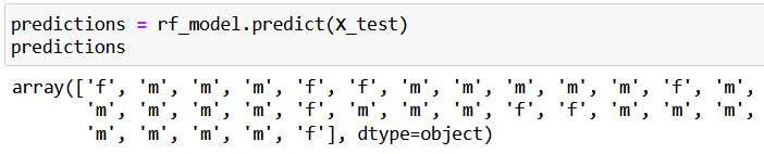
You just give some data (X_test) to your model (rf_model), then call the predict() method too, well, make predictions. The predictions are saved to predictions.

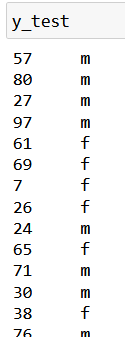
You can compare the predicted values (predictions) to the true values (y_test), if you’re curious:

You can even check the probabilities assigned by your model to each prediction with predict_proba():

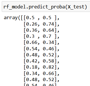
Each array contains two probabilities in this case because we have two categories to predict: male or female. The left value shows the predicted probability of belonging to the category of female, the second shows the same for belonging to the category of male.

How do we know this?

With the help of classes_:

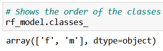
If you’d like to know how important each feature is in predicting a possum’s sex, that’s also possible with feature_importances_:

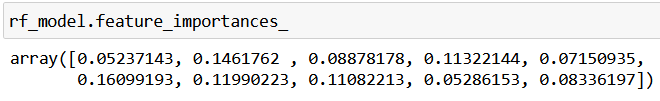
feature_importances_ reflects the order of the columns in your features dataframe so you just need to match its values to the features’ names, like this:

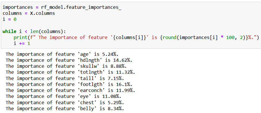
Interesting to see that head length (footlgth) has the highest predicting power (16.1%) in a possum’s sex, isn’t it? 🙂

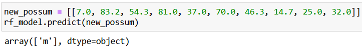
By the way, at this point your random forest model is ready, so feel free to feed any new data to it to make a new prediction:

Conclusion

That’s it. This is how you create a random forest model in Python with scikit-learn. The amazing thing about random forests is that they’re easy to comprehend and can be utilized with great effect without any complicated hyperparameter tuning.

I don’t know if you realized it, but you’ve just acquired some really useful knowledge – or at least I hope so! –, because you’ll come across random forests many times in your machine learning journey.

I do encourage you to read more articles and watch more videos on this topic, because there are still many mind-blowing things to discover! 🙂

• If you want to learn more about how to become a data scientist, take Tomi Mester’s 50-minute video course: How to Become a Data Scientist. (It’s free!)
• Also check out the 6-week online course: The Junior Data Scientist’s First Month video course.

Cheers,
Tamas Ujhelyi