SQL functions (SUM, COUNT, AVG, MIN, MAX) and GROUP BY | SQL for Data Analysis Tutorial, ep3

In this article, I’ll show you the most essential SQL functions that you will use for calculating aggregates — such as SUM, AVG, COUNT, MAX, MIN — in a data set. Then I’ll show you how these work with the GROUP BY clause, so you will be able to use SQL for segmentation projects. (Eg. you’ll learn, how you can calculate averages with GROUP BY in SQL.) Eventually, you’ll learn some intermediate SQL moves using ORDER BY and DISTINCT.

The good news: these things don’t change too much over time. SQL functions and GROUP BY were the same in 2012 as they are today in 2022. So if you learn them now, you’ll be good with that knowledge at least till 2032. 😉

Anyways, you’ll learn a lot of new stuff here… so buckle up — because you have to know all these to efficiently use SQL for data analysis! Oh, and this is going to be super exciting, as we will still use our 7M+ line data set!

Note: to get the most out of this article, you should not just read it, but actually do the coding part with me!

Before we start…

…I recommend going through these articles first – if you haven’t done so yet:

1. Set up your own data server: How to set up Python, SQL, R, and Bash (for non-devs)
2. Install SQL Workbench to manage your SQL queries better: How to install SQL Workbench for PostgreSQL
3. Read the first two episodes of the SQL for Data Analysis series: ep 1 and ep 2
4. Make sure that you have the flight delays data set imported – and if you don’t, check out this article.

SQL functions to aggregate data

Okay, let’s open SQL Workbench and connect to your data server!

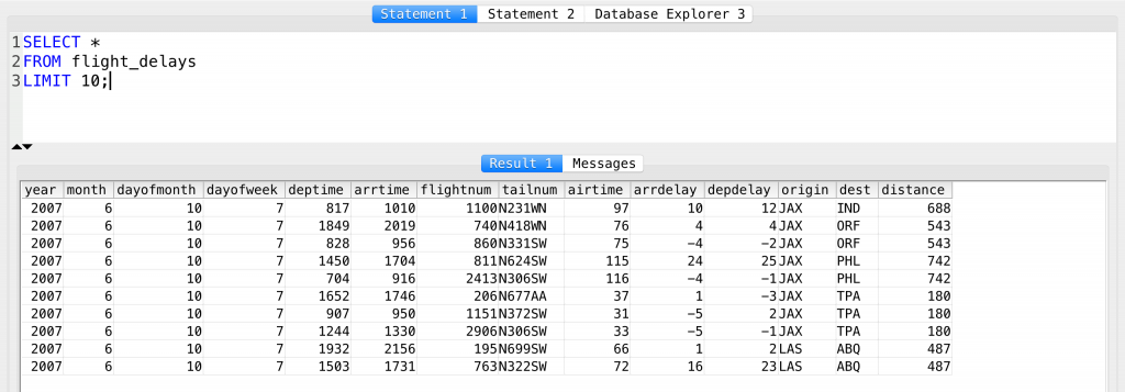
Can you recall our base query?
It was:

SELECT *
FROM flight_delays
LIMIT 10;

And it returned the first 10 lines of this huge data set.

We are going to modify this query to get answers to 5 important questions:

• How many lines are there in our SQL table? (We’ll use the SQL COUNT function for that.)
• What’s the total airtime of all the flights on our table? (That’ll be an SQL SUM function.)
• What’s the average of all arrival delays in the table– and what’s it for all the departure delays? (SQL AVG function.)
• What’s the maximum distance value in our SQL table? (SQL MAX function.)
• What’s the minimum distance value in our SQL table? (SQL MIN function.)

Getting the answers to all these questions is going to be very easy, I promise. But again: make sure you are doing the coding part with me. Coding is the easiest to learn by doing it. So please spare no effort at this point: type in everything you see here into your SQL manager, too, and build a solid foundation of knowledge!

Okay, let’s see this!

SQL COUNT function. Let’s count lines!

The easiest aggregation function is to count lines in your SQL table. And this is what the COUNT function is for. The only thing you have to change – compared to the above base query – is what you SELECT from your table. Remember? It can be everything (*), or it can be specific columns (arrdelay, depdelay, etc). Now, let’s expand this list with functions. Copy this query into SQL Workbench and run it:

SELECT COUNT(*)
FROM flight_delays
LIMIT 10;

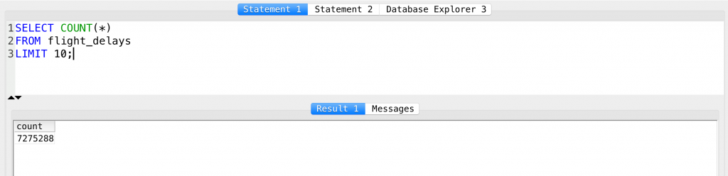
The result is: 7275288.

The function itself is called COUNT, and it says to count the lines using every column (*)… You can change the * to any column’s name (eg. arrdelay) – and you will get the very same number. Try this:

SELECT COUNT(arrdelay)
FROM flight_delays
LIMIT 10;

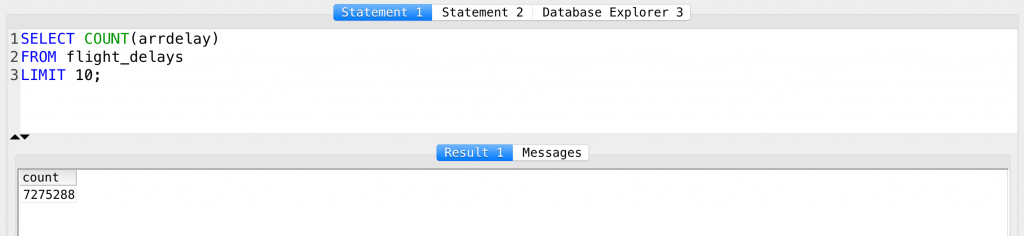
Right? Same result: 7275288.

So yes, this means that we have 7275288 lines in our flight_delays table.

Note 1: This is true only when you don’t have NULL values (empty cells) in your table! (We don’t have NULL values in the flight_delays data set at all.) I’ll get back to the importance of NULL later.
Note 2: in fact, you won’t need the LIMIT clause in this SQL query, as you will have only one line of data on your screen. But I figured that sometimes it might be better to keep it there, so even if you mistype something, your SQL Workbench won’t freeze by accidentally trying to return 7M+ lines of data.

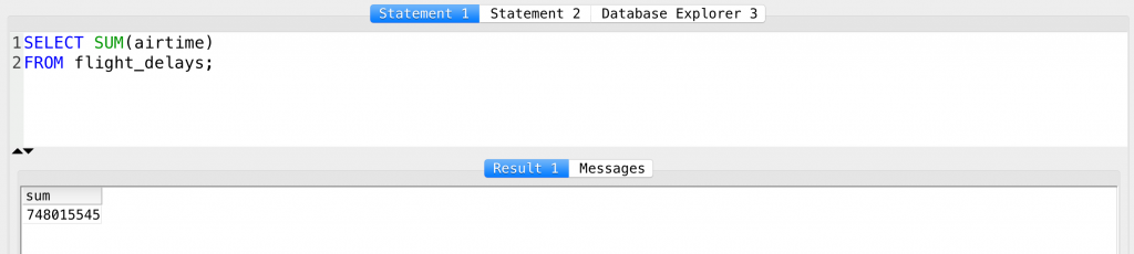
SQL SUM function. Calculate sum!

Now we want to get the airtime for all flights – added up. In other words: get the sum of all values in the airtime column. The SUM function works with a similar logic as COUNT does. The only difference is that in the case of SUM you can’t use * — you’ll have to specify a column. In this case, it’ll be the airtime column.

Try this query:

SELECT SUM(airtime)
FROM flight_delays;

The total airtime is a massive 748015545 minutes.

SQL AVG function. Calculate averages… I mean the *mean*.

Our next challenge is to calculate the average arrival delay value and the average departure delay value. It’s important to know that there are many types of statistical averages in mathematics. But we usually refer to the average type called mean — when we say “average” in everyday life. (A quick reminder: mean is calculated by calculating the sum of all values in a dataset, then dividing it by the number of values.)

In SQL, the function called AVG (which of course stands for “average”) returns the mean… so the average type is what we expect from it.

Note: well, I have to add that many data scientists find it a bit lazy and ambiguous that in SQL the general word of “average” (AVG) is used for one specific average type: mean. And they are right! Median and mode are also averages. In Python/pandas, for example, the function to calculate the mean is actually called mean — and then there is another one called median to calculate median. That’s much more coherent. Well, like it or not, in SQL we have *AVG* for mean.

The syntax and the logic are the same as it was for the previous two SQL functions.

You can try it out by running this query:

SELECT AVG(depdelay)
FROM flight_delays;

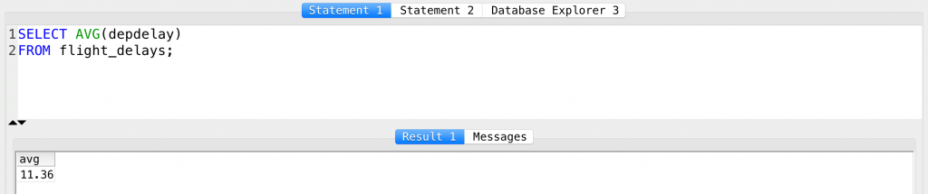
The result is 11.36.

But of course, you’d get the exact same value if you typed:

SELECT SUM(depdelay)/COUNT(depdelay)
FROM flight_delays;

But let’s not run that far ahead… Instead of that, let’s calculate the average arrdelay value, too:

SELECT AVG(arrdelay)
FROM flight_delays;

Result: 10.19

Cool!

SQL MAX and MIN functions. Let’s get maximum and minimum values.

And finally, let’s find the maximum and the minimum values of a given column. Finding the maximum and minimum distances for these flights sounds interesting enough. SQL-syntax-wise, MIN and MAX operate just like SUM, AVG and COUNT did.

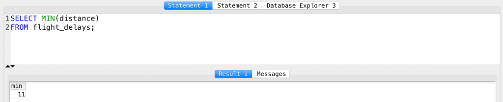
Here’s the minimum distance:

SELECT MIN(distance)
FROM flight_delays;

Result: 11 miles. (Man, maybe take the bike next time.)

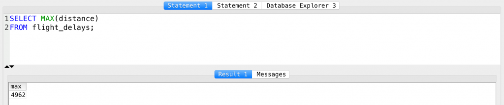
SELECT MAX(distance)
FROM flight_delays;

Result: 4962

Okay! That was it – these are the basic SQL functions you have to know.

• COUNT
• SUM
• AVG
• MAX
• MIN

It wasn’t that difficult so far, so it’s time to tweak this a little bit…

Introducing the GROUP BY clause!

SQL GROUP BY – for basic segmentation analysis and more…

SQL GROUP BY – the theory

As a data scientist, you will probably run segmentation projects all the time. For instance, it’s interesting to know the average departure delay of all flights (we have just learned that it’s 11.36). But when it comes to business decisions, this number is not actionable at all.

However, if we turn this information into a more useful format – let’s say we break it down by airport – it will instantly become something we can act on!

Here’s a simplified chart showing how SQL uses GROUP BY to create automatic segmentation based on column values:

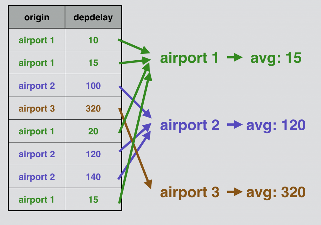
The process has three important steps:

STEP 1 – Specify which columns you want to work with as an input. In our case, we want to use the list of the airports (origin column) and the departure delays (depdelay column).

STEP 2 – Specify which column(s) you want to create your segments from. For us, it’s the origin column. SQL automatically detects every unique value in this column (in the above example these were airport 1, airport 2, and airport 3). Then it creates groups (segments) from them and sorts each line from your data table into the right group.

STEP 3 – Finally it calculates the averages (using the SQL AVG function) for each and every group (segment) and returns the results on your screen.

The only new thing here is the “grouping” at STEP 2. We have an SQL clause for that. It’s called GROUP BY. Let’s see it in action.

SQL GROUP BY – in action

Here’s a query that combines an SQL AVG function with the GROUP BY clause — and does the exact thing that I described in the theory section above:

SELECT
  AVG(depdelay),
  origin
FROM flight_delays
GROUP BY origin;

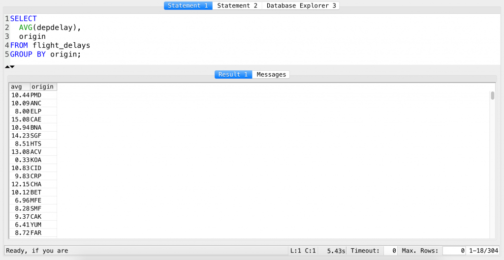
Fantastic!

If you scroll through the results, you will see that there are some airports with an average departure delay of more than 30 or even 40 minutes. From a business perspective, it’s important to understand what’s going on at those airports. On the other hand, it’s also worth taking a closer look at how the good airports (depdelay close to 0) are managing to reach this ideal phase. (Okay, I know, the business case is over-simplified, but you get the point.)

But what just happened SQL-wise?

We have selected two columns – origin and depdelay. origin has been used to create the segments (GROUP BY origin). depdelay has been used to calculate the averages of the arrival delays in these segments (AVG(depdelay)).

Note: As you can see, the logic of SQL is not as linear as it was for Python, pandas, or bash. If you write an SQL query, the first line of it could highly rely on the last line. When you write long and complex queries, this might cause some unexpected errors and thus of course a little headache too… But that’s why I find it very, very important to give yourself enough time to practice the basics and make sure that you fully understand the relationships between the different clauses, functions, and other stuff in SQL.

Test yourself #1 (SQL SUM + GROUP BY)

Here’s a little assignment to practice! Let’s try to solve this task and double-check that you understand everything so far! It’s simple:
Print the total airtime by month!
.
.
.
Ready?
Here’s my solution:

SELECT
  month,
  SUM(airtime)
FROM flight_delays
GROUP BY month;

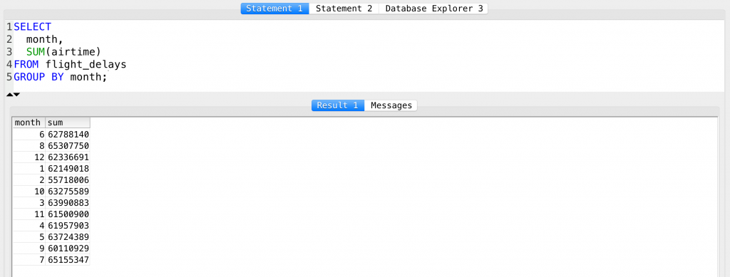
I did pretty much the same stuff that I have done before, but now I’ve created the groups/segments based on the months – and this time I had to use the SUM function instead of AVG.

Test yourself #2 (SQL AVG + GROUP BY)

And here’s another exercise:
Calculate the average departure delay by airport again, but this time use only those flights that flew more than 2000 miles (you will find this info in the distance column).
.
.
.
Here’s the query:

SELECT
  AVG(depdelay),
  origin
FROM flight_delays
WHERE distance > 2000
GROUP BY origin;

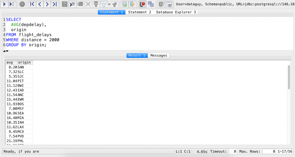
There are two takeaways from this assignment.

1. You might have suspected this but now it’s confirmed: you can use the SQL WHERE clause with GROUP BY and SQL functions.
2. You can filter with WHERE even those columns that are not part of your SELECT statement.

SQL ORDER BY – to sort the data based on the value of one (or more) column(s)

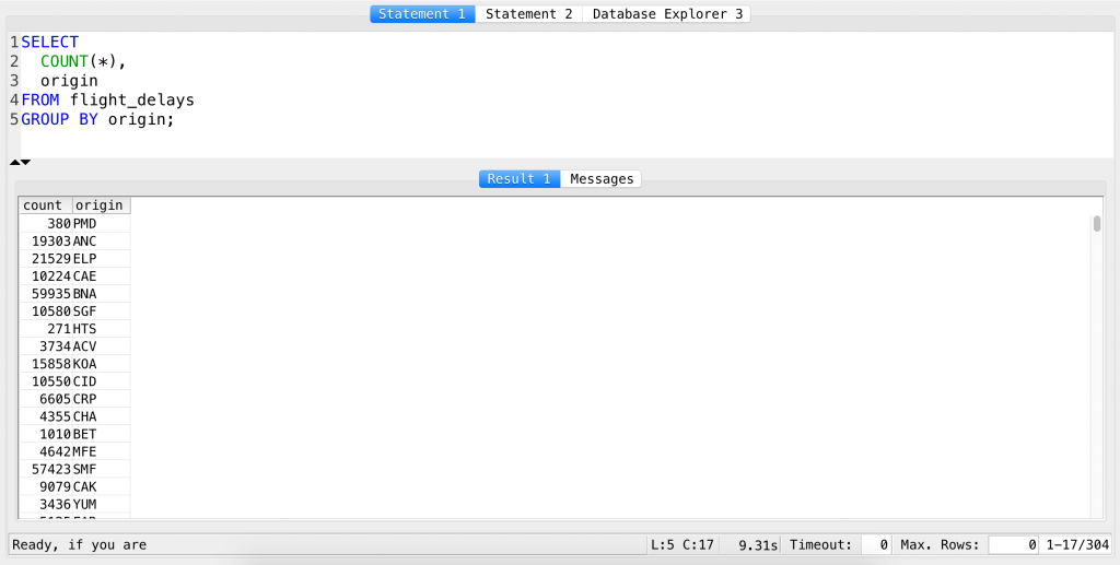
Let’s say we want to see which airport was the busiest in 2007.

You can get the number of departures by airport really easily using the COUNT function with the GROUP BY clause, right? We have done this before in this article:

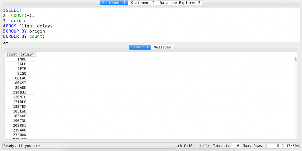
SELECT
  COUNT(*),
  origin
FROM flight_delays
GROUP BY origin;

The problem: this list is not sorted by default… To have that too, you need to add one more SQL clause: ORDER BY. When you use it, you always have to specify which column you want to order by… It’s pretty straightforward:

SELECT
  COUNT(*),
  origin
FROM flight_delays
GROUP BY origin
ORDER BY count;

Note: the column you will get after the COUNT function will be a new column… And it has to have a name – so SQL automatically names it “count” (check the latest screenshot above). When you refer to this column in your ORDER BY clause, you have to use this new name. I’ll get back to this in my next article in detail. If you find it weird, let’s try the same query but with ORDER BY origin – and you will understand it instantly.

Hm, almost there. But the problem is that the least busy airport is on the top – in other words, we got a list in ascending order. That’s the default for ORDER BY (in our PostgreSQL database at least). But you can change this to descending order by simply adding the DESC keyword at the end!

SELECT
COUNT(*),
origin
FROM flight_delays
GROUP BY origin
ORDER BY count DESC;

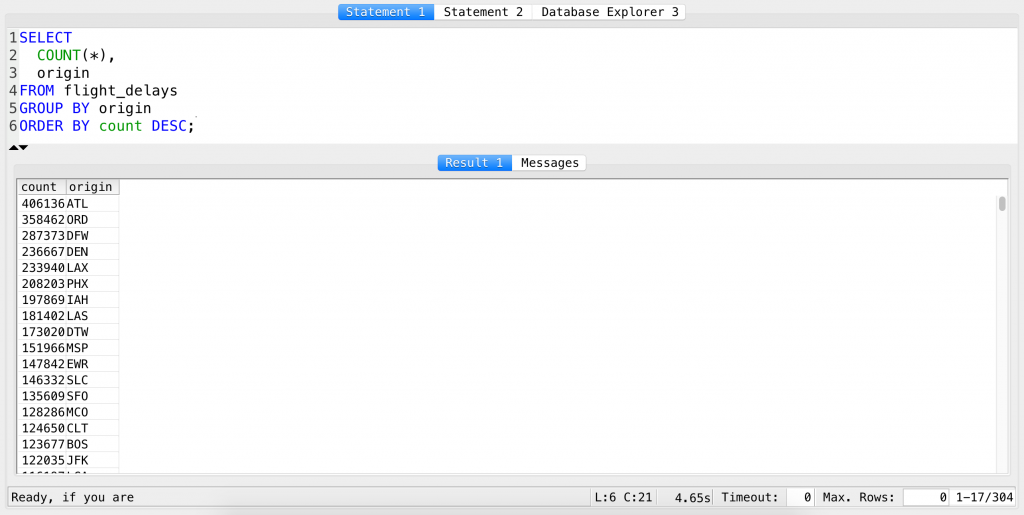
Excellent! Just what we wanted to see!

SQL DISTINCT — to get unique values only

This is the last new thing for today. And this will be short and sweet.

If you are curious how many different airports are in your table:

a) you can find it out using the GROUP BY clause. (Can you figure out how? :-))
b) you can find it out even more easily by using DISTINCT

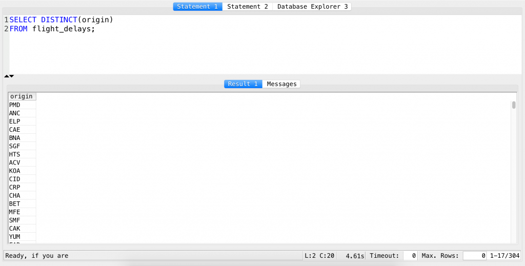
DISTINCT removes all duplicates. Try this:

SELECT DISTINCT(origin)
FROM flight_delays;

Now you have unique airports!

By the way, the GROUP BY version would look like this:

SELECT origin
FROM flight_delays
GROUP BY origin;

Though result-wise it’s pretty much the same, the preferred way to do this is to use the DISTINCT syntax. (When writing more complex queries, DISTINCT will help you to keep your query simpler… But I’ll get back to this in a later article.)

Test yourself #3

Today you have learned a ton of small but useful stuff. I’ll give you one more assignment that will summarize pretty much everything – even the previous two articles (ep 1 and ep 2). This is going to be a difficult one, but you can do it! If it doesn’t work, try to break it down into smaller tasks, then build and test your query until you get the result.
The task is:

List the:

• top 5 planes (identified by the tailnum)
• by the number of landings
• at PHX or SEA airport
• on Sundays

(eg. if the plane with the tailnumber 'N387SW' landed 3 times in PHX and 2 times in SEA in 2007 on any Sunday, then it has a total of 5. And we need the top 5 planes with the higher total.) Ready? Set! Go!
.
.
.
Done? Here’s my solution:

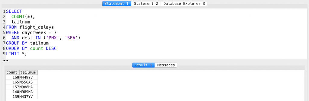
SELECT
  COUNT(*),
  tailnum
FROM flight_delays
WHERE dayofweek = 7
  AND dest IN ('PHX', 'SEA')
GROUP BY tailnum
ORDER BY count DESC
LIMIT 5;

And some explanation:

• SELECT –» select…
• COUNT(*), –» This function counts the number of rows in a given group; to do that it needs the GROUP BY clause later.
• tailnum –» This will help to specify the groups (referred in the GROUP BY function later).
• FROM flight_delays –» the name of the table, of course
• WHERE dayofweek = 7 –» a filter for Sundays only
• AND dest IN ('PHX', 'SEA') –» filter for PHX and SEA destinations only
• GROUP BY tailnum –» This is the clause that helps us to put the lines into different groups by tailnumbers.
• ORDER BY count DESC –» and let’s order by the number of lines in a given group
• LIMIT 5; –» list only the top 5 elements.

Conclusion

And that’s it! You have learned a lot today – SQL aggregate functions (MIN, MAX, COUNT, SUM, AVG), GROUP BY and two more important SQL clauses (DISTINCT and ORDER BY).

If you managed to get the last exercise done by yourself, I can tell you that you have a really good basic knowledge of SQL! Congrats! If not, don’t worry, just make sure that you re-read these first 3 chapters (ep 1, ep 2, ep 3) before you continue with episode 4!

• If you want to learn more about how to become a data scientist, take my 50-minute video course: How to Become a Data Scientist. (It’s free!)
• Also check out my 6-week online course: The Junior Data Scientist’s First Month video course.

Cheers,
Tomi Mester

Cheers,
Tomi Mester