
Let’s continue with the pandas tutorial series! This is the second episode, where I’ll introduce pandas aggregation methods — such as count(), sum(), min(), max(), etc. — and the pandas groupby() function. These are very commonly used methods in data science projects, so if you are an aspiring data scientist, make sure you go through every detail in this article… because you’ll use these probably every day in real-life projects.
Note 1: This is a hands-on tutorial, so I recommend doing the coding part with me!
Before we start
If you haven’t done so yet, I recommend checking out these articles first:
- How to install Python, R, SQL, and bash to practice data science
- Python for Data Science – Basics #1 – Variables and basic operations
- Python Import Statement and the Most Important Built-in Modules
- Top 5 Python Libraries and Packages for Data Scientists
- Pandas Tutorial 1: Pandas Basics (Reading Data Files, DataFrames, Data Selection)
Aggregation – in theory
Aggregation is the process of turning the values of a dataset (or a subset of it) into one single value. Let me make this clear! If you have a pandas DataFrame like…
| animal | water_need |
| zebra | 100 |
| lion | 350 |
| elephant | 670 |
| kangaroo | 200 |
…then a simple aggregation method is to calculate the sum of the water_need values, which is 100 + 350 + 670 + 200 = 1320. Or a different aggregation method would be to count the number of the values in the animal column, which is 4. The theory is not too complicated, right?
So let’s see the rest in practice!
Pandas aggregation methods (in practice)
Where did we leave off last time? We opened a Jupyter notebook, imported pandas and numpy and loaded two datasets: zoo.csv and article_reads. We will continue from there – so if you have no idea what I’ve just talked about in my previous sentence, move over to this article: pandas tutorial – episode 1!
If you are familiar with the basics, for your convenience, here are the datasets we’ll use again:
zoodataset: 46.101.230.157/datacoding101/zoo.csvarticle_readsdataset: 46.101.230.157/dilan/pandas_tutorial_read.csv
Ready? Cool!
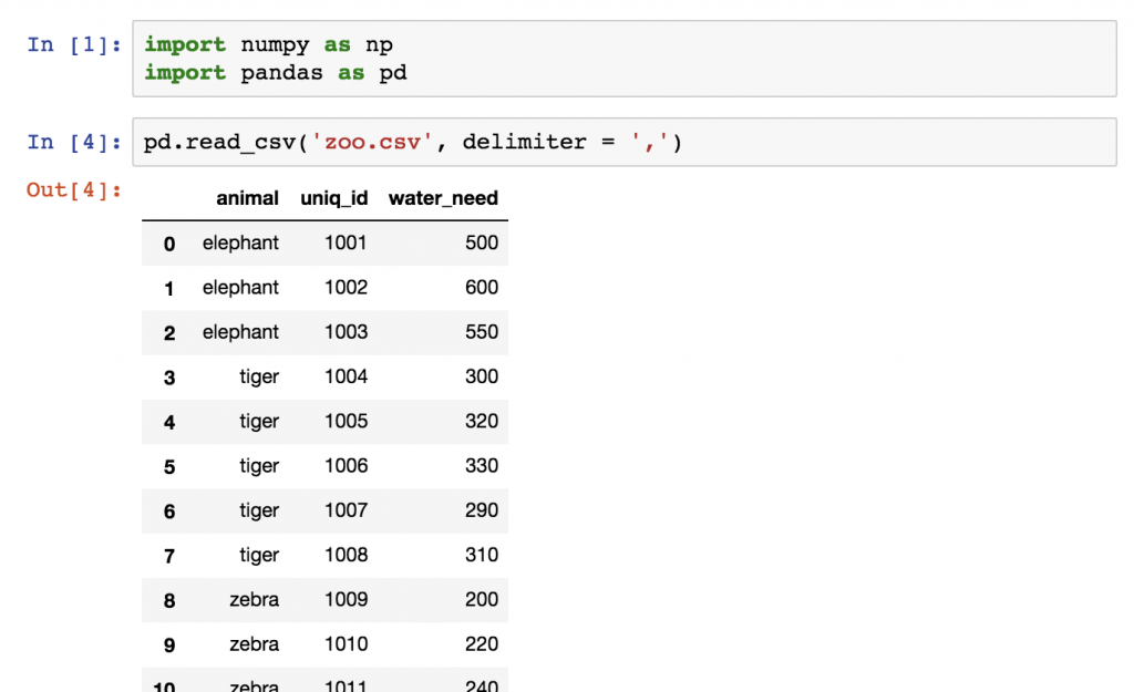
Let’s start with our zoo dataset! (If you want to download it again, you can find it at this link.) We have loaded it by using:
pd.read_csv('zoo.csv', delimiter = ',')
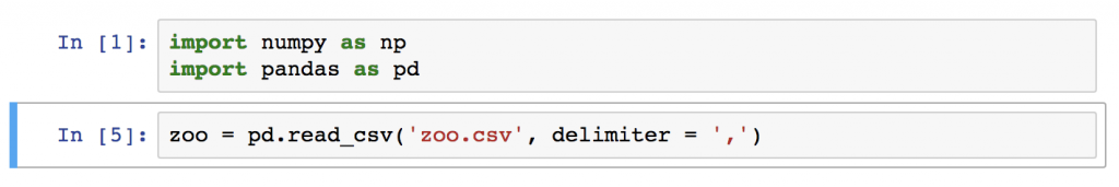
Let’s store this dataframe into a variable called zoo.
zoo = pd.read_csv('zoo.csv', delimiter = ',')
To learn the basic pandas aggregation methods, let’s do five things with this data:
- Let’s count the number of rows (the number of animals) in
zoo! - Let’s calculate the total
water_needof the animals! - Let’s find out which is the smallest
water_needvalue! - And then the greatest
water_needvalue! - And eventually the average
water_need!
Note: for a start, we won’t use the groupby() method but don’t worry, I’ll get back to that when we went through the basics.
#1 pandas count()
The most basic aggregation method is counting. To count the number of the animals is as easy as applying a count pandas function on the whole zoo dataframe:
zoo.count()
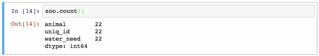
That’s interesting. “What are all these lines?” – you might ask…
Actually, the pandas .count() function counts the number of values in each column. In the case of the zoo dataset, there were 3 columns, and each of them had 22 values in it.
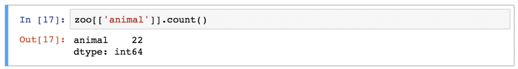
If you want to make your output clearer, you can select the animal column first by using one of the selection operators (that we learned about in the previous article). Something like this:
zoo[['animal']].count()
Or in this particular case, the result could be even nicer if you use this syntax:
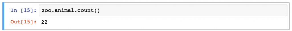
zoo.animal.count()
This also selects only one column, but it turns our pandas dataframe object into a pandas series object. And the count function will be applied to that. (Which means that the output format is slightly different.)
#2 sum() in pandas
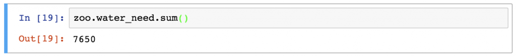
Following the same logic, you can easily sum the values in the water_need column by typing:
zoo.water_need.sum()
Just out of curiosity, let’s run our .sum() function on all columns, as well:
zoo.sum()
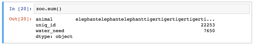
Note: I love how .sum() turns the words of the animal column into one string of animal names. (By the way, it’s very much in line with the logic of Python.)
Pandas Data Aggregation #3 and #4: min() and max()
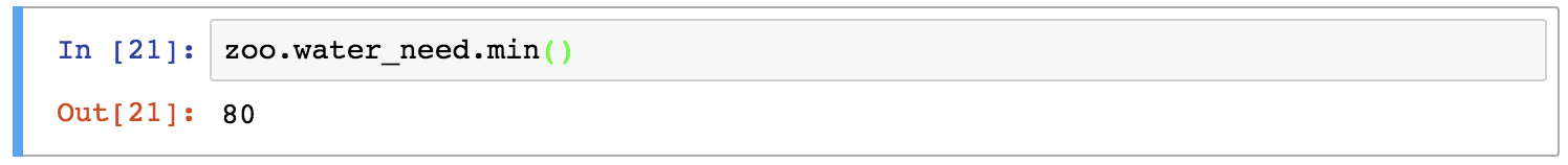
How to make pandas return the smallest value from the water_need column?
I bet you have figured it out already:
zoo.water_need.min()
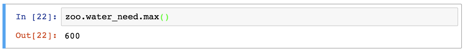
And getting the max value works pretty similarly:
zoo.water_need.max()
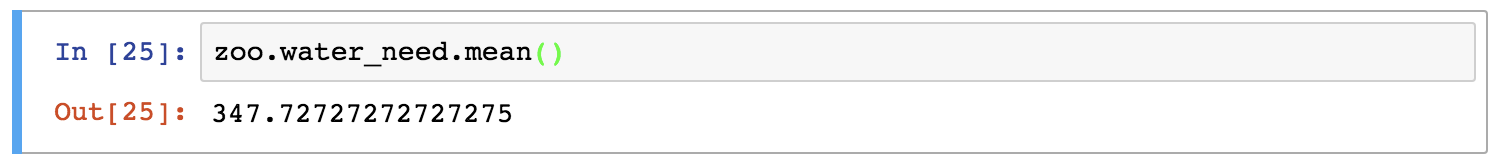
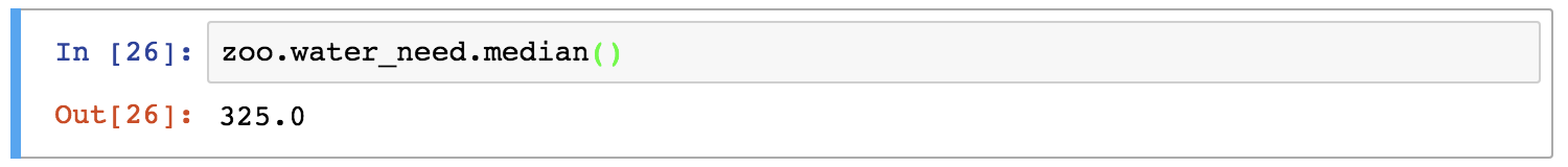
#5: averages in pandas: mean() and median()
Eventually, let’s calculate statistical averages, like mean and median!
The syntax is the same as it was with the other aggregation methods above:
zoo.water_need.mean()
zoo.water_need.median()
Okay, this was easy, right? Pandas aggregation methods are much, much easier than SQL’s, for instance.
So it’s time to spice this up — with a little bit of grouping! Introducing the groupby() function!
The pandas groupby() function (aka. grouping in pandas)
As a data scientist, you will probably do segmentations all the time. For instance, it’s nice to know the mean water_need of all animals (we have just learned that it’s 347.72). But very often it’s much more actionable to break this number down – let’s say – by animal types. With that, we can compare the species to each other. (Do lions or zebras drink more?) Or we can find outliers! (Elephants drink a lot!)
Here’s a simple visual showing how pandas performs “segmentation” – with groupby and aggregation:
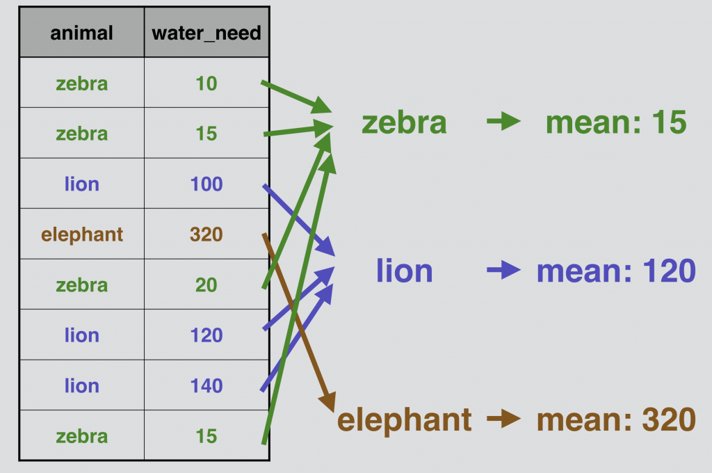
It’s just grouping similar values and calculating the given aggregate value (in the above example it was a mean value) for each group.
Pandas groupby() – in action
Let’s do the above-presented grouping and aggregation for real, on our zoo DataFrame!
We have to fit in a groupby keyword between our zoo variable and our .mean() function:
zoo.groupby('animal').mean()
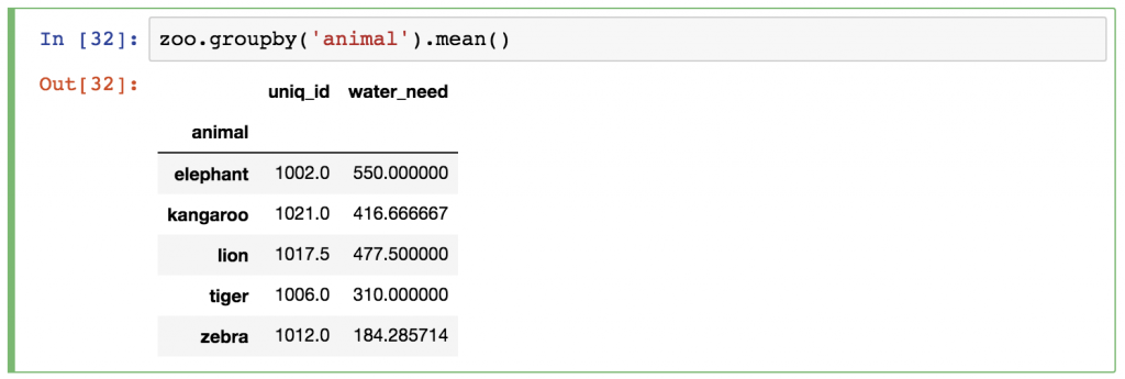
Just as before, pandas automatically runs the .mean() calculation for every column (the animal column disappeared since that was the column we grouped by). You can either ignore the uniq_id column or you can remove it afterward by using one of these syntaxes:
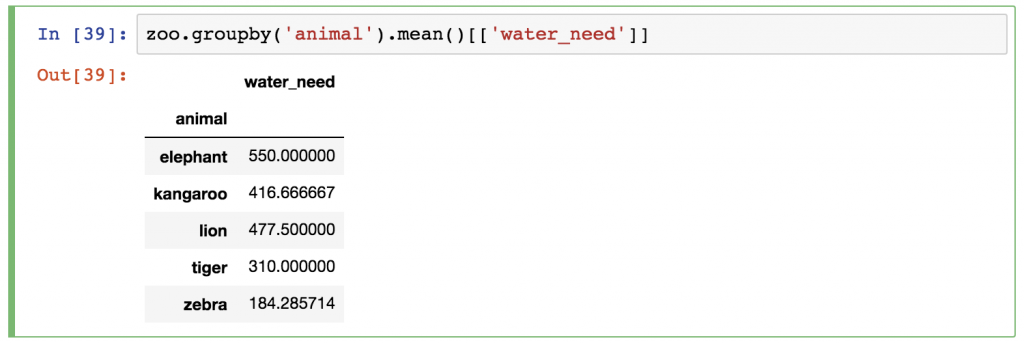
zoo.groupby('animal').mean()[['water_need']] –» This returns a DataFrame object.
zoo.groupby('animal').mean().water_need –» This returns a Series object.
Obviously, you can change the aggregation method from .mean() to anything, we learned above!
Let’s see one more example and combine pandas groupby and count!
Pandas groupby() and count()
I just wanted to add this example because it’s the most common operation you’ll do when you discover a new dataset. Using count and groupby together is just as simple as the previous example was.
Just type this:
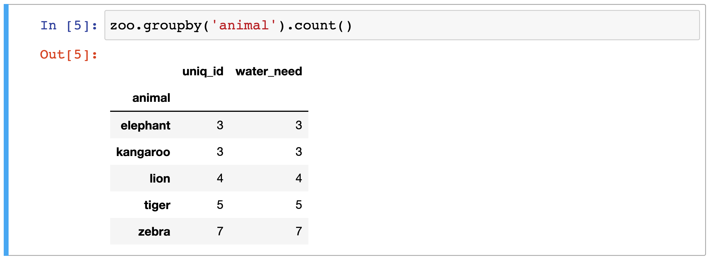
zoo.groupby('animal').count()
And magically the different animals are counted by pandas:
Okay! Now you know everything, you have to know!
It’s time to…
Test yourself #1 (another count + groupby challenge)
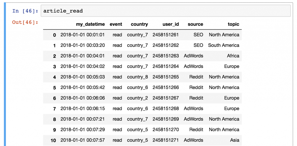
Let’s get back to our article_read dataset.
(Note: Remember, this dataset holds the data of a travel blog. If you don’t have the data yet, you can download it from here. Or you can go through the whole download-open-store process step by step by reading the previous episode of this pandas tutorial.)
If you have everything set, here’s my first assignment:
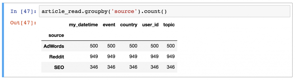
What’s the most frequent source in the article_read dataframe?
.
.
.
And the solution is Reddit!
How did I get it? Use this code:
article_read.groupby('source').count()
I’ll break it down for you:
- Take the
article_readdataset! - Use
groupby()and create segments by the values of thesourcecolumn! - And eventually, count the values in each group by using
.count()after thegroupby()part.
You can – optionally – remove the unnecessary columns and keep the user_id column only, like this:
article_read.groupby('source').count()[['user_id']]
Test yourself #2
Here’s another, slightly more complex challenge:
For the users of country_2, what was the most frequent topic and source combination? Or in other words: which topic, from which source, brought the most views from country_2?
.
.
.
The result is the combination of Reddit (source) and Asia (topic), with 139 reads!
And the Python code to get this result is:
article_read[article_read.country == 'country_2'].groupby(['source', 'topic']).count()
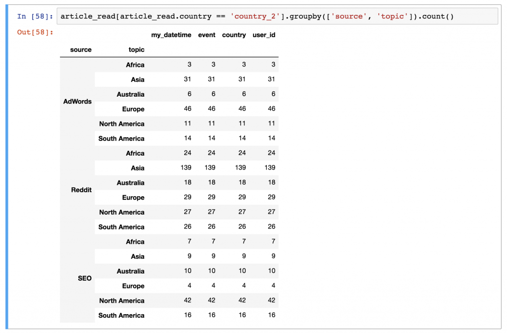
Here’s a brief explanation:
- First, we filtered for the users of
country_2witharticle_read[article_read.country == 'country_2'] - Then on this subset, we applied a
groupbypandas method… Oh, did I mention that you can group by multiple columns? Now you know that, too! 😉 (Syntax-wise, watch out for one thing: you have to put the name of the columns into a list. That’s why the bracket frames go between the parentheses.) (That was thegroupby(['source', 'topic'])part.) - And as per usual: the
count()function is the last piece of the puzzle.
Conclusion (pandas groupby, count, sum, min, max, etc.)
This was the second episode of my pandas tutorial series. Now you see that aggregation and grouping are not too hard in pandas… and believe me, you will use them a lot!
Note: If you have used SQL before, I encourage you to take a break and compare the pandas and the SQL methods of aggregation. With that, you will understand more about the key differences between the two languages!
In the next article, I’ll show you the four most commonly used pandas data wrangling methods: merge, sort, reset_index and fillna. Stay with me: Pandas Tutorial, Episode 3!
- If you want to learn more about how to become a data scientist, take my 50-minute video course: How to Become a Data Scientist. (It’s free!)
- Also check out my 6-week online course: The Junior Data Scientist’s First Month video course.
Cheers,
Tomi Mester
Cheers,
Tomi Mester
PS. for a detailed guide, check out pandas’ official guide (it’s very updated — last refreshed in 2022), here.