Regression Tree in Python Using Scikit-learn (Code Your Decision Tree Part #1)

The title says it all: in this article, you’ll learn how to code regression trees with scikit-learn.

Before you continue, I advise you to read this and this article to familiarize yourself with some predictive analytics and machine learning concepts. Please also make sure that you have matplotlib, pandas, and scikit-learn installed. Other than that, you’re all set up. 😎

If you don’t have your Python environment for data science, go with one of these options to get one:

• Get your own data server and install the most popular data science libraries
• Install Anaconda on your local computer

The most important definitions about decision trees

I’m pretty sure you’ve already seen a decision tree. Like this:

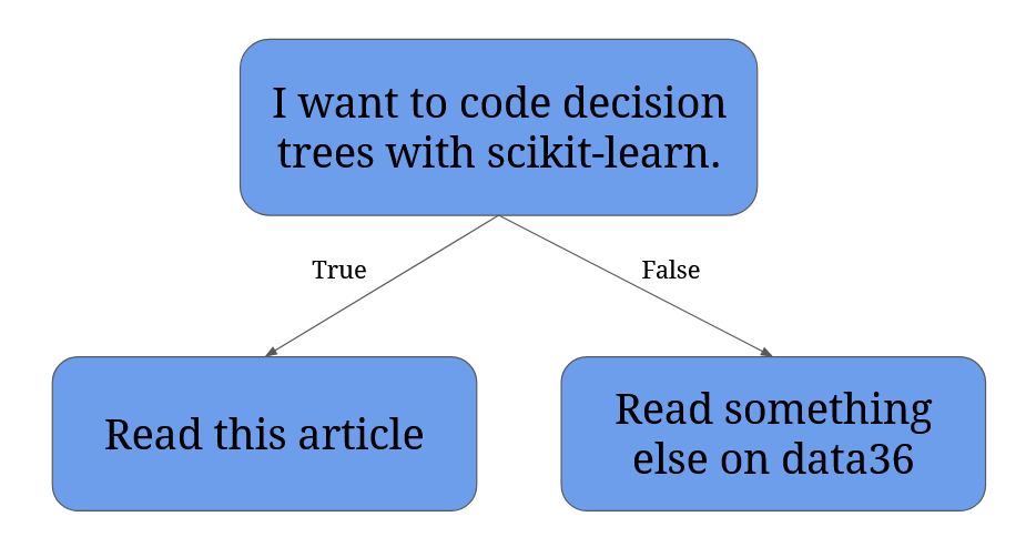
Decision trees can also be much bigger. Like this:

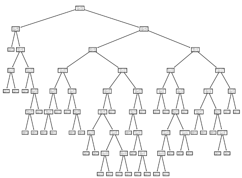
(Spoiler: you’ll create the exact same tree soon.)

What do you see in the second image?

• A bunch of rectangles, called nodes. Nodes are important, because they contain statements, like “I want to code decision trees with scikit-learn.”
• One lonely node at the very top. It’s called the root node.
• Nodes at the bottom without any arrows pointing from them. These are the leaf nodes. Leaf nodes contain the output values or final decisions (like “Read this article”).
• Lots of arrows. Arrows represent decisions based on the evaluation of a node’s statement. Usually, left-pointing arrows represent “True”, while right-pointing arrows represent “False”.
• Parent/child nodes: if two nodes are connected with an arrow, they have a relationship. If a node has an arrow pointing from it, it’s a parent node. If a node has an arrow pointing towards it, it’s a child node. A node can be both a parent and a child node.
• Split/splitting: when a statement is evaluated in a node, and as a result, two arrows point out of it towards two new nodes. The “I want to code decision trees with scikit-learn.” example is a split.
• Pruning: when you make your tree shorter, for instance because you want to avoid overfitting. (Okay, you’ve caught me red-handed, because this one is not in the image. But I’ve already started this bullet points thing, and I really didn’t want to break the pattern. Sorry for that.)

Anyway. If you throw around terms like “split” or “leaf node” next time you discuss decision trees with your friends, you’ll sound like a proper person who knows his/her stuff.

One more thing. When we use a decision tree to predict a number, it’s called a regression tree. When our goal is to group things into categories (=classify them), our decision tree is a classification tree.

In this article, we’ll create both types of trees. Let’s start with the former.

Coding a regression tree I. – Downloading the dataset

In machine learning lingo a regression task is when we want to predict a numerical value with our model. You may have already read about two such models on this blog (linear regression and polynomial regression).

This time we’ll create a regression tree to predict a numerical value. We’ll use the Possum Regression dataset from Kaggle made available by ABeyer. As stated on the dataset’s page by its uploader:

“Data originally found in the DAAG R package and used in the book Maindonald, J.H. and Braun, W.J. (2003, 2007, 2010) “Data Analysis and Graphics Using R”).

A subset of the data was also put together for the OpenIntro Statistics book chapter 8 Introduction to linear regression.

Original Source of dataset:

Lindenmayer, D. B., Viggers, K. L., Cunningham, R. B., and Donnelly, C. F. 1995. Morphological variation among columns of the mountain brushtail possum, Trichosurus caninus Ogilby (Phalangeridae: Marsupialia). Australian Journal of Zoology 43: 449-458.”

You can download the dataset by clicking on the download button:

The possum dataset contains data about 104 possums:

• sex,
• age,
• head length,
• skull width,
• etc.

We’ll create a regression tree to predict the age of possums based on certain characteristics of the animals.

Coding a regression tree II. – Exploring and preparing the data

First, import pandas and matplotlib:

import pandas as pd
import matplotlib.pyplot as plt

Then save the dataset into a dataframe (df), and display its first five rows (df.head()):

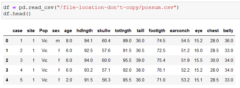
(Don’t blindly copy the above code, use the path where your file is located!)

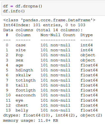
Let’s make a quick overview of our data with df.info():

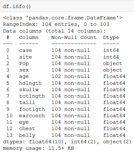
We can conclude that:

• we have 104 rows (104 possums),
• there are 14 columns,
• two columns (age and footlgth) have missing values (we know this because they don’t have 104 non-null values),
• most columns store numerical values (either float64 or int64).

We could try to estimate the missing values, but for this tutorial, we’ll just remove any rows that have a missing value with dropna(), and save the remaining rows into df:

df = df.dropna()

A second df.info() shows that we’re left with 101 rows to work with. But before we can start coding our regression tree, we do some more cleaning by removing columns that don’t contain morphometric measurements:

X = df.drop(["case", "site", "Pop", "sex", "age"], axis=1)
y = df["age"]

After this step, X stores the features (the inputs based on which our regression tree will predict the age of the possums), and y stores only the ages of the possums (the numerical values we wish to predict with our regression tree).

The importance of saving the features and the age values into X and y will become clear in a second:

from sklearn.model_selection import train_test_split
X_train, X_test, y_train, y_test = train_test_split(X, y, test_size=0.3, random_state=44)

With the help of the train_test_split method, we split all of our X and y values into training (X_train, y_train) and test (X_test, y_test) groups – 30% of all data goes to the test groups (test_size=0.3), and 70% goes to the training groups.

I advise you to use random_state=44 so your code will allocate the exact same (=with the same index label) feature and age values from X and y.

Note: Here’s an explanation as to why that is with random_state.

Coding a regression tree III. – Creating a regression tree with scikit-learn

The wait is over. 🙂 Let’s celebrate it by importing our Decision Tree Regressor (the stuff that lets us create a regression tree):

from sklearn.tree import DecisionTreeRegressor

Next, we create our regression tree model, train it on our previously created train data, and we make our first predictions:

model = DecisionTreeRegressor(random_state=44)
model.fit(X_train, y_train)
predictions = model.predict(X_test)

Some explanation:

model = DecisionTreeRegressor(random_state=44) >> This line creates the regression tree model.

model.fit(X_train, y_train) >> Here we feed the train data to our model, so it can figure out how it should make its predictions in the future on new data.

predictions = model.predict(X_test) >> Finally, we instruct our model to predict the ages of the possums that can be found in X_test (remember, our model has not seen the data in X_test before, so it’s completely new in its eyes!).

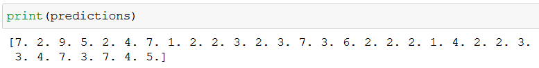
If you print predictions, you’ll see the age values our model estimates for the possums in X_test:

Just to see the full picture, the rows in X_test look like this:

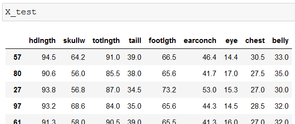
If you compare the two above images, you can see that our model predicted the first possum in X_test (row 57) to be 7 years old. The second possum (row 80) is estimated to be only 2 years old. And so on…

We also have the true age values in y_test:

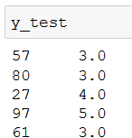
Armed with predictions and y_test, you can calculate the performance of your model with the root mean square error (RMSE). You can read how under the “STEP #3: Creating a polynomial regression model” section in this article about polynomial regression.

What’s more important now is that you can feed any data into your model, and it’ll estimate the age of a possum (in the below example I’ve used the data for the row with index 37):

You can also plot your regression tree (but it’s more interesting with classification trees, so I’ll explain this code in more detail in the later sections):

from sklearn.tree import plot_tree
plt.figure(figsize=(10,8), dpi=150)
plot_tree(model, feature_names=X.columns);

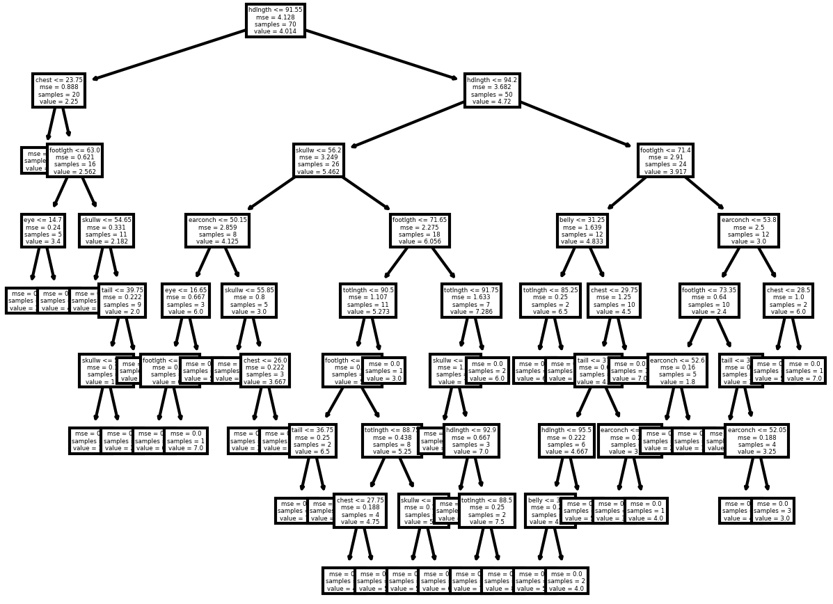
For now, don’t worry too much about what you see. What’s important is that now you know how to predict a numerical value with a regression tree, but keep in mind that regression trees are usually not used for making numerical estimations!

Conclusion

I’d like to let you in on a little secret – there’s much more to decision trees than regression trees. Of course, now you can code regression trees, which is nice, but in the next article, I’ll show you something beautiful: how you can create classification trees. (It’ll be much more fun, pinky promise! 😉)

• If you want to learn more about how to become a data scientist, take Tomi Mester’s 50-minute video course: How to Become a Data Scientist. (It’s free!)
• Also check out the 6-week online course: The Junior Data Scientist’s First Month video course.

Cheers,
Tamas Ujhelyi