
You can’t get enough of decision trees, can you? 😉 If coding regression trees is already at your fingertips, then you should definitely learn how to code classification trees – they are pure awesomeness! Not only that, but in this article, you’ll also learn about Gini Impurity, a method that helps identify the most effective classification routes in a decision tree.
A few prerequisites: please read this and this article to understand the basics of predictive analytics and machine learning. Also, install matplotlib, pandas, and scikit-learn so you can seamlessly code along with me.
If you don’t have your Python environment for data science, go with one of these options to get one:
- Get your own data server and install the most popular data science libraries
- Install Anaconda on your local computer
A warmup thought experiment to classification trees
Let’s say your cousin runs a zoo housing exclusively tigers and zebras. Let’s also say your cousin is really bad at animals, so they can’t tell zebras from tigers apart. 😔
Now imagine a situation where some of the tigers and zebras break loose. Here’s the problem: some tigers are dangerous, because they are young and full of energy, so they would love to hunt down the zebras (the older tigers know they regularly get food from the zookeepers, so they don’t bother hunting).
Zookeepers are out searching for the escaped animals. If they see one, they immediately call your cousin in the headquarters to ask what they should do with the animal:
- if it’s a zebra, they lure it back to its place with grass,
- if it’s a normal tiger, they entice it back to its place with a meatball,
- if it’s a dangerous tiger, they capture it with a special net (then take it back to the tigers).
For understandable reasons, your cousin wants to identify all animals as soon as possible. But they have very limited knowledge about them:
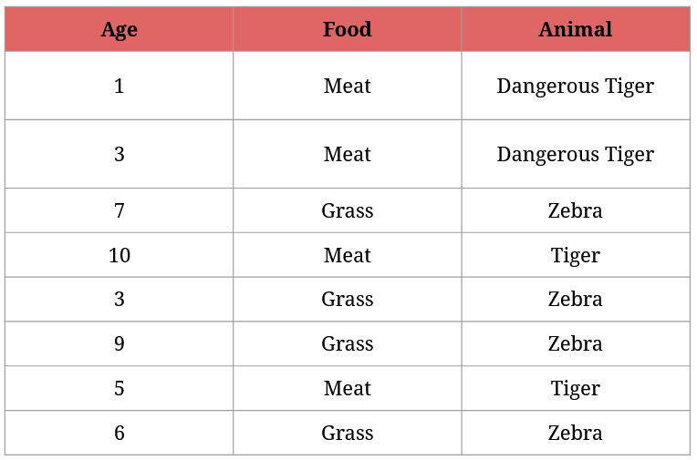
What questions should your cousin ask from the zookeepers to asap identify the animals?
You can try to come up with a solution yourself, but there’s an approach classification trees use to solve problems like this. It’s called Gini Impurity.
Wait.
Gini what?
What is Gini Impurity and how to calculate it?
Gini Impurity is one of the most commonly used approaches with classification trees to measure how impure the information in a node is. It helps determine which questions to ask in each node to classify categories (e.g. zebra) in the most effective way possible.
Its formula is:
1 - p12 - p22
Or:
1 - (the probability of belonging to the first category)2 - (the probability of belonging to the second category)2
(The formula has another version too, but it’ll yield the same results.)
Gini Impurity is at the heart of classification trees; its value is calculated at every split, and the smaller number we get, the better. A smaller number means that the split did a great job at separating the different classes.
A classification tree’s goal is to find the best splits with the lowest possible Gini Impurity at every step. This ultimately leads to 100% pure (=containing only one type of categorical value, e.g. only zebras) leaf nodes.
Let’s walk through some examples to understand this concept better.
Calculating Gini Impurity for categorical values
Getting back to your cousin and the escaped animals, they could ask first whether an animal eats meat:
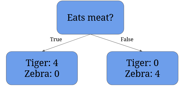
This split results in two nodes: the left node contains all tigers (even the dangerous ones), the right node contains only the zebras.
Now we can calculate the Gini Impurity for each node:
- Right node’s Gini Impurity:
1 - (probability of belonging to tigers)2 - (probability of belonging to zebras)2=1 - 12 - 02 = 1 - 1 - 0 = 0 - Left node’s Gini Impurity:
1 - (probability of belonging to tigers)2 - (probability of belonging to zebras)2=1 - 02 - 12 = 1 - 0 - 1 = 0
A Gini Impurity of 0 means there’s no impurity, so the data in our node is completely pure. Completely pure means the elements in the node belong to only one category (e.g. all of them are zebras).
There could be a case where we’re totally unsure which category an element belongs to: if we have four zebras and four tigres in a node, it’s a 50-50 situation. In such cases Gini Impurity is 0.5. (Which is: 1 - 4/82 - 4/82 = 1 - 0.52 - 0.52 = 1 - 0.25 - 0.25 = 0.5)
We’ve seen two examples for calculating a node’s Gini Impurity. But there exists a Gini Impurity value for the whole split as well. To calculate it, we have to take the weighted average of the nodes’ Gini Impurity values:
- let’s count first how many elements we have in total:
8(4tigers and4zebras), - then count how many elements we have in each node (left:
4, right:4), - then divide these numbers by the total number of elements, and multiply them by the corresponding node’s Gini Impurity value (left:
4/8 * 0, right:4/8 * 0), - and add them up:
4/8 * 0 + 4/8 * 0 = 0.
The result is 0 because with one question we managed to fully separate zebras and tigers. Your cousin still doesn’t know how to identify the dangerous tigers, though. 😭
If you’d like to help her/him, read further.
Calculating Gini Impurity for continuous/numerical values
We know that any tiger that’s younger than 4 years is considered dangerous:
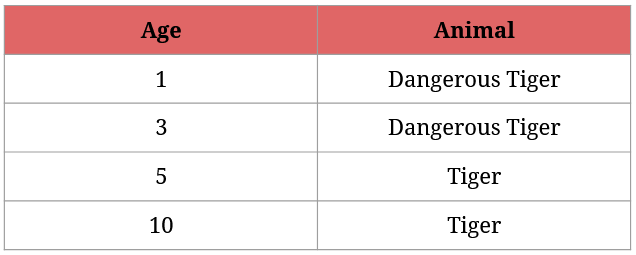
I presume that you immediately know how we could identify the dangerous tigers, but it serves as a good example in explaining how Gini Impurity works with continuous values.
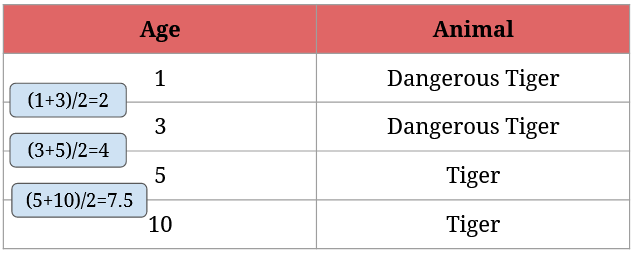
So here’s how the best split is determined with numerical values:
- order the numerical data in increasing order (it’s already done in the above screenshot),
- take the average of every two neighboring numbers,
- then calculate the Gini Impurity for the averages,
- finally, choose the one with the lowest Gini Impurity value.
Here’s what step 2 looks like:
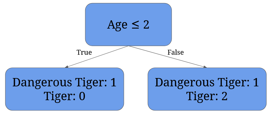
After we have the averages, we need to calculate each possible split’s Gini Impurity value. For 2 it’s given by 1/4 * (1 - 12 - 02) + 3/4 * (1 - 1/32 - 2/32) = 0 + 3/4 * 0.44 = 0.33:
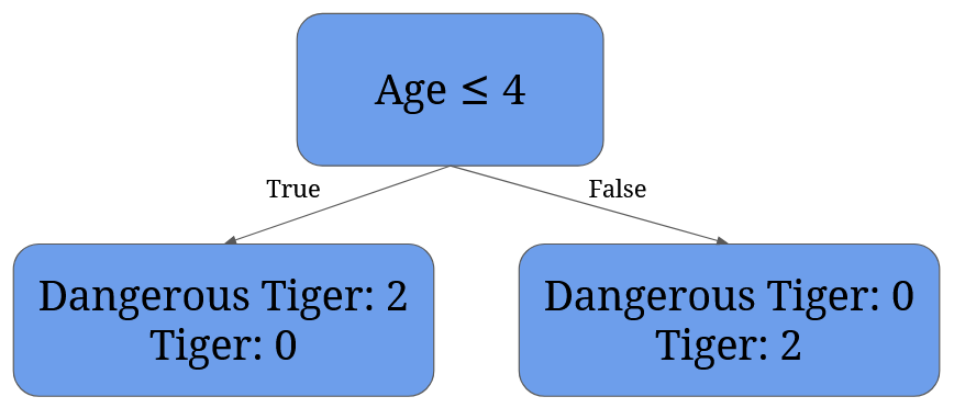
For 4 it’s given by 2/4 * (1 - 12 - 02) + 2/4 * (1 - 02 - 12)= 0:
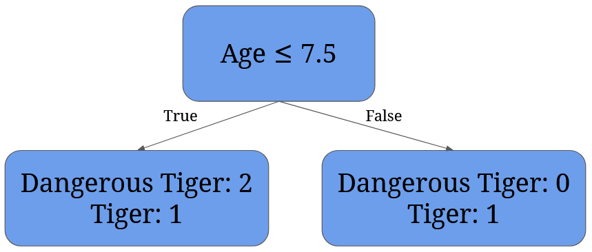
For 7.5 it’s given by 3/4 * (1 - 2/32 - 1/32) + 1/4 * (1 - 02 - 12) = 3/4 * 0.44 + 0 = 0.33:
It’s easy to see that the best split is split at 4 – it perfectly separates dangerous tigers from normal tigers.
With this, we conclude what you should suggest to your cousin: first ask if the animal eats meat, then ask if it’s less than 4 years old.
Now that we know how Gini Impurity is calculated for both categorical and numerical values, it’s time to code our first classification tree.
Let’s code a Decision Tree (Classification Tree) in Python!
Coding a classification tree I. – Preparing the data
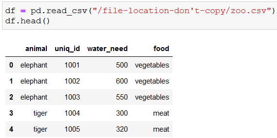
We’ll use the zoo dataset from Tomi Mester’s previous pandas tutorial articles. It’s only a few rows (22) but will be perfect to learn how to build a classification tree with scikit-learn.
We’ll use our tree to predict the species of an animal given its water need and the type of food it favors.
You can download the dataset here. (Full link: 46.101.230.157/datacoding101/zoo_python.csv)
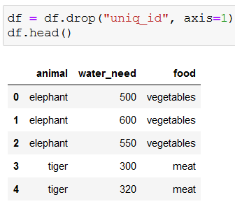
For starters, let’s read in and check out the first five rows of the data:
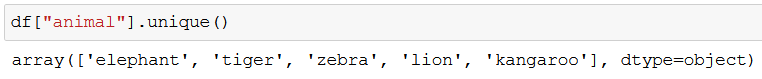
With unique() we can check what kind of animals we’re dealing with:
We won’t need the ids, so let’s drop that column:
Because the decision trees in scikit-learn can’t work with string values, we need to convert strings to numbers with get_dummies():
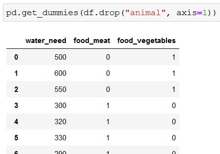
df.drop("animal", axis=1) removes the animal column from our dataframe (df), so get_dummies() is left to work with water_need and food. But since it affects only columns with strings, and water_need stores numerical values, get_dummies() converts only the values of food to numerical values. While doing so, it creates two new columns (food_meat and food_vegetables).
Here’s how to read the two new columns:
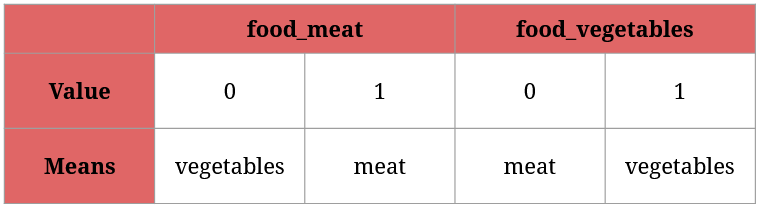
Since food_meat and food_vegetables can’t hold the same value for a given animal (can’t be both 1 or 0; an animal eats either meat or vegetables), using one of them will suffice. For instance, food_meat = 0 and food_vegetables = 1 means the same thing: this animal feeds on vegetables.
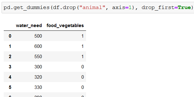
To get rid of one of the columns we use drop_first=True:
pd.get_dummies(df.drop("animal", axis=1), drop_first=True)
As a result, food_meat gets deleted:
Now we’re ready to create our classification tree.
Coding a classification tree II. – Define the input and output data, and split the dataset
We start with these few lines:
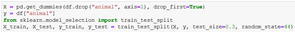
X = pd.get_dummies(df.drop("animal", axis=1), drop_first=True)
y = df["animal"]
from sklearn.model_selection import train_test_split
X_train, X_test, y_train, y_test = train_test_split(X, y, test_size=0.3, random_state=44)
Everything we’ve just done in the previous section, we save to X. X holds the features (also called predictors) for our machine learning model.
Similarly, y holds (y = df["animal"]) the animals, aka the responses that our classification tree will predict: whether a given animal based on its water need and the type of food it eats is an elephant, tiger, etc.
Then we import train_test_split (third line) to save 70% of our features and responses into X_train and y_train respectively, and the rest 30% into X_test and y_test (test_size=0.3 takes care of all of this in the fourth line).
This is a necessary step in machine learning because we want to train our model only on one part of our data, then check its performance on never before seen data (the test data).
And as the last touch, random_state=44 just makes sure that you’ll receive the same results as I if you code along with me.
Here’s the screenshot of what we’ve done so far; nothing spectacular yet, but believe me, we’re getting there:
Coding a classification tree III. – Creating a classification tree with scikit-learn
Now we can begin creating our classification tree model:
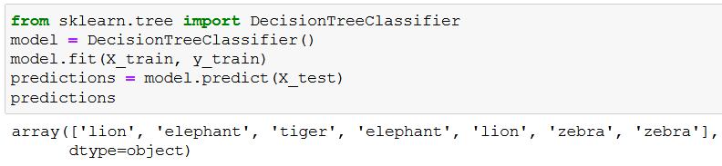
from sklearn.tree import DecisionTreeClassifier
model = DecisionTreeClassifier()
model.fit(X_train, y_train)
predictions = model.predict(X_test)
predictions
Here’s what’s happening:
from sklearn.tree import DecisionTreeClassifier: this import makes it possible for us to create a classification tree,model = DecisionTreeClassifier(): we create our basic classification tree model,model.fit(X_train, y_train): we train our tree on our data reserved for training (X_trainandy_train),- then we give our model data that it never saw before (
predictions = model.predict(X_test)), - and check out what it predicts (
predictions).
Low and behold, the predictions:
We can evaluate the accuracy of these predictions if we check y_test (the variable that holds the true values for the corresponding X_test rows):
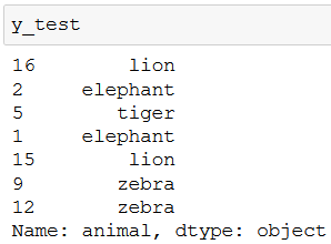
As you can see, our model pretty much nailed it. 🥳
An interesting side note: feature_importances_ shows the relative importance of each feature in a model’s prediction:
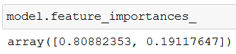
If you add up the two values you get 100% – so the screenshot tells us that while predicting an animal, one feature was much more valuable (almost 81%) than the other (19%). But which one exactly?
Let’s find out with X_train.columns:
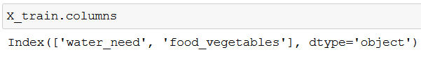
Because feature_importances_ follows the order of columns, we can easily see that water_need plays a more significant role in identifying what kind of animal we are dealing with.
Our tree is finalized, so let’s visualize it!
Coding a classification tree IV. – Visualizing a classification tree
We can visualize our tree with a few lines of code:
from sklearn.tree import plot_tree
plt.figure(figsize=(10,8), dpi=150)
plot_tree(model, feature_names=X.columns, filled=True);
First, we import plot_tree that lets us visualize our tree (from sklearn.tree import plot_tree).
Then we set the size (figsize=(10,8)) and the sharpness (dpi=150) of our visualization: plt.figure(figsize=(10,8), dpi=150).
And finally, we plot our tree with plot_tree(model, feature_names=X.columns, filled=True);:
modelis our already existing tree,feature_names=X.columnsmakes it possible for us to see the names of the features,filled=Truecolors our nodes,- and
;removes any written information that would normally accompany our visualization, so we only get to see our beautiful tree.
Here’s what we’ve been waiting for, our classification tree visualized:
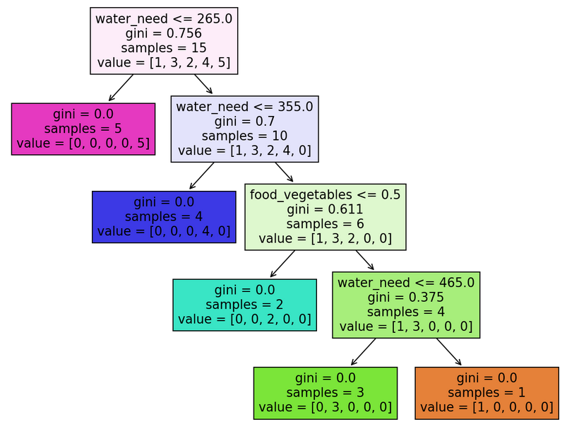
Coding a classification tree V. – What do these all mean?
There are many things to absorb. Let me explain by taking the root node as an example:
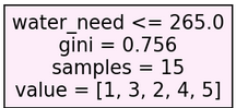
There are four pieces of information in it: water_need, gini, samples and value:
water_need: it doesn’t necessarily have to be water_need (there’s a node with food_vegetables instead). This information shows what feature a given node was split on – if the feature is accompanied with a number (e.g.water_need <= 265.0), it means that our classification tree split the node on a given value of a feature.gini: the Gini Impurity of the node.samples: the number of available elements in a particular node. In the root node’s case, it’s15because we have originally trained our model on 15 animals (X_trainandy_train). The number of samples reduces as we go down the tree, and the tree successfully categorizes the animals.value: if you add the numbers up, you get a number equal to the samples (e.g.[1, 3, 2, 4, 5] = 15). It represents the number of elements in the different categories in a node: for instance[1, 3, 2, 4, 5]means 1 elephant, 3 kangaroos, 2 lions, 4 tigers, and 5 zebras (you can quickly check it withy_train.value_counts()).
A few farewell notes:
- we’ve worked with a very small dataset, so our classification tree made use of all features – it is not often the case with larger datasets and more features, because not every feature is needed to correctly classify categorical values,
- we used Gini Impurity to quantify the impurity of the nodes, but we could have used entropy as well (we used Gini Impurity because it’s a common practice to do so, and it is computationally more efficient),
- with larger datasets and trees you may see the need to prune your tree; you have many settings at your disposal to do so (e.g. using
max_depthormax_lead_nodes).
Conclusion
Huh… it’s been quite a journey, hasn’t it? 😏 I’ll be honest with you, though. Decision trees are not the best machine learning algorithms (some would say, they’re downright horrible).
But don’t let this discourage you, because you’ve done something amazing if you’ve completed this article – you’ve learned the basics of a new machine learning algorithm, and it’s not something to be taken lightly.
So stay tuned, because in the next article we’ll show you how you make decision trees into a powerful random forest algorithm. Until then, keep practicing and share with us the beautiful decision trees you’ve created!
- If you want to learn more about how to become a data scientist, take Tomi Mester’s 50-minute video course: How to Become a Data Scientist. (It’s free!)
- Also check out the 6-week online course: The Junior Data Scientist’s First Month video course.
Cheers,
Tamas Ujhelyi