Predictive Analytics 101 – Part 1

Predictive analytics is not a new or very complicated field of science. As I mentioned before, it’s easy for anyone to understand at least the essence of it.

Imagine that you are in the grocery store. You are done and ready to pay. But which line you choose? Your brain starts to run a built-in “predictive algorithm” with these parameters:

1. Expected output: the fastest line
2. Target variable: time spent in the line (the less the better) – fastest way to leave the shop and go home
3. Historical data: your past experience from previous shopping sessions
4. Predictors (or “features”): length of line, number of items in the baskets, average age of customers in the line, etc…
5. The predictive model: the process your brain goes through while calculating

Basically computers are doing the exact same thing when they do predictive analytics (or even machine learning). They copy how our brain works. Obviously computers are more logical. They use well-defined mathematical and statistical methods and much more data. (Sometimes even big data. The real big data. Not the kind that media folks use all the time to make you click their articles. ;-)) And eventually they can give back more accurate results. At the end of these two articles (Predictive Analytics 101 Part 1 & Part 2) you will learn how predictive analytics works, what methods you can use, and how computers can be so accurate. Don’t worry, this is a 101 article; you will understand it without a PhD in mathematics!

Note: if you are looking for a more general introduction to data science introduction, check out the data analytics basics first!

Why does every business need Predictive Analytics? A possible answer is: Customer Lifetime Value.

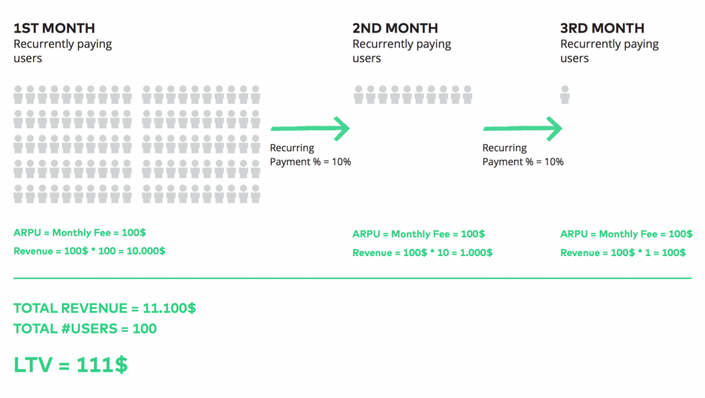
Though it’s not very difficult to understand, predictive analytics is certainly not the first step you take on when you set up the data driven infrastructure of your startup or e-commerce business. You start with KPIs and data research. In a little while you will reach a point where you need to understand another important metric related to your online business. This is the Customer Lifetime Value. At Practical Data Dictionary, I’ve already introduced a very simple way to calculate CLTV. That was:

Download the full 54 pages of the Practical Data Dictionary PDF for free.

It’s a good start, but I’d raise an argument with Past Me. I wrote:
“In this formula, we are underestimating the CLTV. When calculating the CLTV, I would advise underestimating it – if we are thinking in terms of money, it’s better to be pleasantly surprised rather than disappointed!”

That’s not quite true, past Tomi. For instance, if you underestimate the Customer Lifetime Value, you will also underestimate your projected marketing budget. And with that the CPC limits and the overall acceptable Customer acquisition costs. You will spend less. This means you will grow slower. Means you’ll lose potential users. And if you are surrounded with competitors, this could easily cost you your business.

Of course, this is too dramatic. In 95% of the cases you can use the Practical Data Dictionary formula very well and you will be a very happy business owner with a nice profit at the end of the year.
But you would be even happier if your business could grow faster, right? To reach that goal you can’t underestimate nor overestimate your CLTV. You need to know it exactly. This is one important point where predictive analytics can come into play in your online business.

Note: There are many other ways to use predictions for startups/e-commerce businesses. You can predict and prevent churn, you can predict the workload of your support organization, you can predict the traffic on your servers, etc…

How does predictive analytics work in real life?

Step 1 – Select the target variable!

In my grocery store example, the metric we wanted to predict was the time spent waiting in line. If a computer could have done this prediction, we would have gotten back an exact time-value for each line. In this case the question was “how much (time)” and the answer was a numeric value (the fancy word for that: continuous target variable).

There are other cases, where the question is not “how much,” but “which one”. Say you are going to the shop and you are able to choose between black, white, or red T-shirts. The computer will try to predict which one you will choose, maybe recommend you something. It does this based on your historical decisions. In this case the predicted value is not a number, but a name of a group or category (“black T-shirt”). This is a so called “categorical target variable” resulting from a “discrete choice”.

So if you predict something it’s usually:

A) a numeric value (aka. continuous target variable), that answers the question “how much” or
B) a categorical value (aka. categorical target variable or discrete choice), that answers the question “which one”.

These will become important when you are choosing your prediction model.
Anyhow: at this point your focus is on selecting your target variable. You will need to consider business as much as statistics.

Note: there are actually more possible types of target variables, but as this is a 101 article, let’s go with these two, since they are the most common.

Step 2 – Get your historical data set!

If you did the data collection right from the very beginning of your business, then this should not be an issue. Remember the “collect-everything-you-can” principle. When it comes to predictions, it’s extremely handy if you logged everything: now you can try and use lots of predictors/features in your analysis. Most of them won’t play a significant role in your model. But some of them will – and you won’t know which one until you test it out.

It’s also worth mentioning that 99.9% of cases your data won’t be in the right format. At this step you also need to spend time cleaning and formatting your data. But this part is very case-specific, so I leave this task to you.

The concept of overfitting

The idea behind predictive analytics is to “train” your model on historical data and apply this model to future data.

As Istvan Nagy-Racz, co-founder of Enbrite.ly, Radoop and DMLab (three successful companies working on Big Data, Predictive Analytics and Machine Learning) said:

“Predictive Analytics is nothing else, but assuming that the same thing will happen in the future, that happened in the past.”

Let’s take an example. You have dots on your screen, blues and reds. The screen has been generated by a ruleset that you don’t know; you are trying to find it out. You see some kind of correlation between their position on the screen and their color.

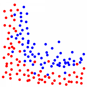
A new dot shows up on the screen. You don’t know the color, only the position. Try to guess the color!

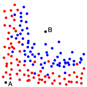
Of course if the dot is in the upper right corner, you will say it’s most probably blue. (dot B)
And if it’s the left bottom corner, you will say it’s most probably red. (dot A)

That’s what a computer would say, but it works with a mathematical model, not with gut feelings. The computer try to come up with a curve that splits the screen. One side is blue, the other side is red. But what does the exact curve look like?

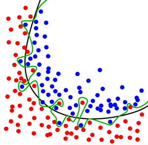
There are several solutions. The black and green curves above are two of those. Which model is the most accurate? You would say the green one, right? It has 0% error and 100% accuracy. Unfortunately there is a high chance that you are wrong.

The green-line prediction model includes the noise as well, and the accuracy is 100% in this case. However if you regenerate the whole screen, it’s very likely that you will have a similar screen, but with different random errors. You will see that the green line model’s accuracy will be much worse in this new case (let’s say 70%).

The black line model has only 90% accuracy, but it doesn’t take into consideration the noise. It’s more general, so its accuracy will be 90% again if you regenerate the screen with different random errors.

That’s what we in predictive analytics call the overfitting issue.
Here’s another great example of overfitting:

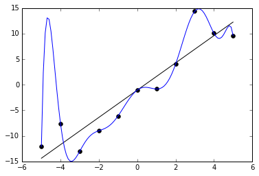
Right? The black-line looks like a better model for nice predictions in the future – the blue looks like overfitting.

Both cases show that the more general the model is, the better. But that’s the theory. In real life you can never know. That’s why you need as a next step…

Step 3 – Split your data!

We usually split our historical data into 2 sets:

1. Training set: the dataset that we use to teach our model.
2. Test set: the dataset that we use to validate our model before using it on real life future data.

The split has to be done with random selection, so the sets will be homogeneous. It’s obvious, but worth mentioning, that the bigger the historical data set is, the better the randomization and the prediction will be.

But what’s the right split? 50%-50%? 80%-20%? 20%-80%? 70%-30%?
Well, that could be another whole blog article. There are so many methods and opinions.

Most people – at least most people I know – focus more on the training part, so they assign 70% of the data to the training set and 30% to the test set. This is called the holdout method.

Some others make 3 sets: training, fine-tuning and test sets. So they train the model with the training set, they fine-tune it with the fine-tuning set and eventually validate it with the test set.

What I like the most is a method called Monte Carlo cross-validation – and not only because of the name. In this process you basically repeatedly select 20% portions (or any X%) of your data. You select 20%, use it for any of the training/validation/testing methods, then drop it. Then select another random 20%. The selections are independent from each other in every round. This means you can use the same data points several times. The advantage of it is that you can run these rounds infinite times, so you can boost your accuracy round by round.

So all in all:
1. Train the model! (And I’ll dig into the details in Part 2 of Predictive Analytics 101.)
2. Validate it on the test set.
And if the training set and test set give back the same error % and the accuracy is high enough, you have every reason to be happy.

To be continued…

UPDATE! Here’s Part 2: LINK!
I will continue from here next week. The next steps will be:
Step 4 – Pick the right prediction model and the right features!
Step 5 – How do you validate your model?
Step 6 – Implement!
Bonus – when predictive analytics fails…

Plus I’ll add some personal thoughts about the relationship between big data, predictive analytics and machine learning.

Continue with Part 2 here.

• If you want to learn more about how to become a data scientist, take my 50-minute video course: How to Become a Data Scientist. (It’s free!)
• Also check out my 6-week online course: The Junior Data Scientist’s First Month video course.

Cheers,
Tomi Mester

Cheers,
Tomi Mester