Beautiful Soup Tutorial 4. – Saving Scraped Data to a CSV File, then Analyzing it with Pandas

This is the final part of the Beautiful Soup tutorial series. Just to remind you, here’s what you’ve done so far:

• in episode #1 you learnt the basics of Beautiful Soup and Requests by scraping your first web page and extracting some basic information from the web page’s HTML content,
• in episode #2 you scraped more web pages, created a pandas dataframe from the scraped data, and visualized your insights (bar chart, box plot),
• in episode #3 you really outdid yourself by scraping more than 1,000 product pages; you also learnt some more advanced aspects of web scraping (user-agents, headers parameter) to bypass web servers that want to block scraping activities.

And now, your final journey awaits – you’ll learn how to save scraped data to a CSV file, so you can access it later whenever you want. And because you’re someone who’s after valuable knowledge, you’ll also learn how to extract interesting insights from your gathered data.

If it sounds interesting to you, I urge you to keep on reading.

Saving scraped data to a CSV file

After you’ve run your code, you’ll have a bestseller_books list containing all bestsellers with information about them.

Let’s create a dataframe out of this list:

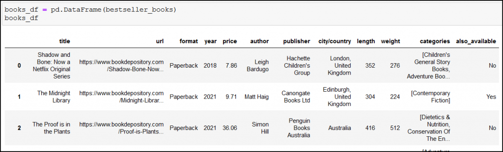
You should have 10 pieces of information (which is 10 columns) about your books.

Note: in the screenshot you can see two more additional columns (weight, also_available), but don’t worry about them, it’ll be an extra challenge for you, if you’re up to it – more on that at the end of the article.

Because we don’t want to lose our precious scraped data, it’s best that we save it to a CSV file:

books_df.to_csv("/home/user_name/books_df.csv", index=False)

You can freely set the path and the name of the file, so don’t blindly copy the above line, feel free to save your CSV according to your preferences. index=False is needed, because our dataframe already has an index column.

Loading the .csv file with pandas

Once you’ve created a CSV file, you can easily load it with pandas’ pd.read_csv() method:

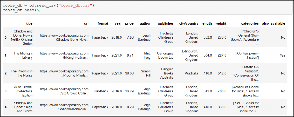
After loading the data, you may immediately notice two things:

1. the year and the length values changed from integer to float (for example from 352 to 352.0); don’t worry about it, it’s just something that happens when you save/load data with pandas to/from a CSV file,
2. long values got truncated (just look at the first URL, it ends with “…”).

This second one is a real issue! We want to see the full values, otherwise we can’t do proper analyses (look again at the first row, but now at the categories column: not all categories are being shown).

What’s the solution? An easy setting:

pd.set_option('display.max_colwidth', None)

Here’s the result:

Full values, yesss! *party music on*

We finally have our data properly loaded, so let’s celebrate it with some quick analyses. 🙂

Analyzing bestseller authors – Who is the most popular writer?

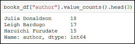
Are you curious which top 3 authors have the most titles in Book Depository’s bestsellers list? I certainly am.

Run:

books_df["author"].value_counts().head(3)

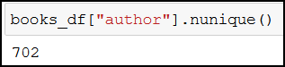
How many authors made it to the bestsellers list? It’s:

books_df["author"].nunique()

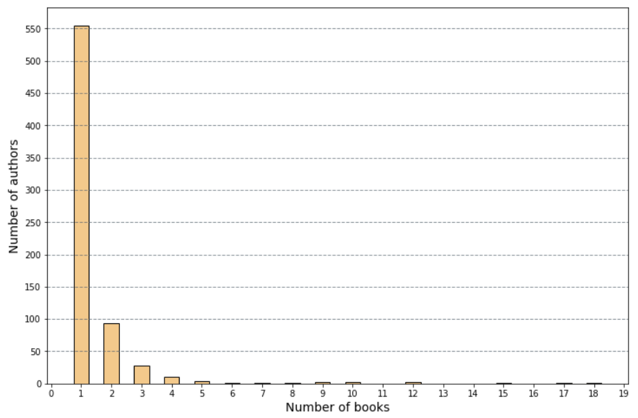
The below bar chart also shows us that out of the 702 authors, most of them (550+) only have 1 book in the bestsellers list:

The code for the bar chart:

books_by_author = books_df["author"].value_counts().value_counts().to_frame().reset_index()
books_by_author.rename(columns={"index":"number_of_books", "author":"number_of_authors"}, inplace=True)
plt.figure(figsize=(12, 8))
plt.yticks(np.arange(0, 600, step=50))
plt.xticks(np.arange(0, 20, step=1))
plt.ylabel("Number of authors", fontsize = 14)
plt.xlabel("Number of books", fontsize = 14)
plt.bar(books_by_author["number_of_books"], books_by_author["number_of_authors"], width = 0.5, color = "#F3C98B", edgecolor = "black")
plt.grid(color='#59656F', linestyle='--', linewidth=1, axis='y', alpha=0.7)

(Don’t freak out if you have different results, because Book Depository’s bestseller list is updated daily.)

Analyzing bestseller publishers and publication cities/countries

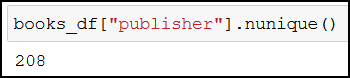
How many publishers are present with their publications in the bestsellers list?

books_df["publisher"].nunique()

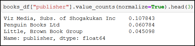
Which top 3 publishers have the most books in the list?

books_df["publisher"].value_counts().head(3)

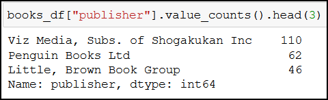
It’s also interesting that around 20% of the bestsellers are published by the top 3 publishers (0.10% + 0.06% + 0.04%).

books_df["publisher"].value_counts(normalize=True).head(3)

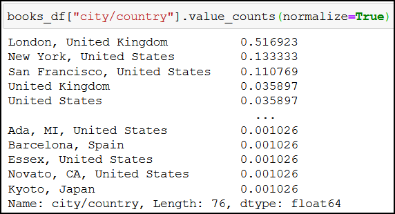
And around 51% of the bestsellers are published in London, United Kingdom:

books_df["city/country"].value_counts(normalize=True)

Analyzing categories on product pages

Let’s find out typically how many categories bestsellers are categorized into:

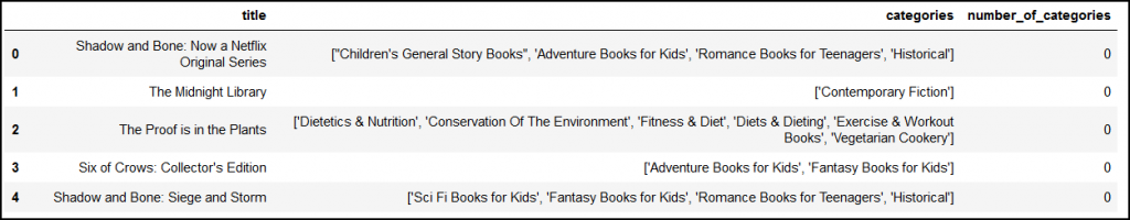
categories_df = books_df[["title", "categories"]]
categories_df.insert(loc=2, column="number_of_categories", value=0)
categories_df.head(5)

We create a new dataframe (categories_df), where we only keep the title and the categories columns (books_df[["title", "categories"]]). Then we create a new column after our already existing categories column, name it number_of_categories, and give it a value of 0. The first 5 rows of the new dataframe will look similar to this:

Converting strings to lists

Take a closer look at the values of the categories column: they may look like lists, but in reality they’re strings (because we loaded our original books_df dataframe from a CSV file) – let’s turn them into real lists!

The following piece of code turns our list-looking-strings into lists:

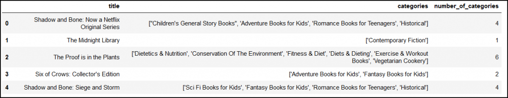
categories_df["categories"] = categories_df["categories"].map(lambda x: x.strip("][").split(", "))
categories_df["number_of_categories"] = categories_df.apply(lambda x: len(x["categories"]), axis="columns")

The categories_df["categories"].map(lambda x: x.) part means that something will happen to every value (denoted by x) in the categories column. That something is this:

• first we remove the square brackets from our string (.strip("][")),
• then we create a list from our string by defining that list elements are separated by “, “ in our string (.split(", ")),
• and as a last touch we give real values to number_of_categories, by determining the length of the lists (created in the previous step) in categories (categories_df.apply(lambda x: len(x["categories"]), axis="columns")).

Here’s what we’ve done:

Counting the values and visualizing the results

Now we know exactly how long each list is (how many categories a given book is categorized into). From here, we can easily count how many books are categorized into how many categories (we’ve already done these steps with other data during this tutorial series,  so I won’t explain them again):

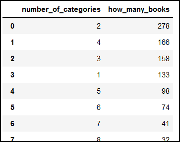
categories_df = categories_df["number_of_categories"].value_counts().to_frame().reset_index()
categories_df.rename(columns={"index":"number_of_categories", "number_of_categories":"how_many_books"}, inplace=True)

This is what we get running the code:

We can also visualize this data:

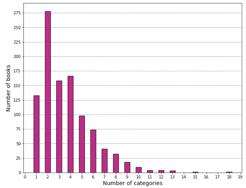
Now we have a more visually appealing way to show that most bestsellers are categorized into only 2 categories! 🙂

As always, here’s the code for the bar chart:

plt.figure(figsize=(10, 8))
plt.yticks(np.arange(0, 300, step=25))
plt.xticks(np.arange(0, 20, step=1))
plt.ylabel("Number of books", fontsize = 14)
plt.xlabel("Number of categories", fontsize = 14)
plt.bar(categories_df["number_of_categories"], categories_df["how_many_books"], width = 0.5, color = "#BD2D87", edgecolor = "black")
plt.grid(color='#59656F', linestyle='--', linewidth=1, axis='y', alpha=0.7)

Creating a frequency distribution of bestseller books’ length

This section may be a bit statistical, so feel free to jump to the conclusion. But if you’re interested, read on.

Here’s the plan: we’ll create a frequency distribution of the bestseller books’ length, but first we’ll remove outliers from our data following the steps outlined by codebasics in his excellent video.

Let’s first find the mean value of the length of the books:

length_mean = books_df["length"].mean()
length_mean

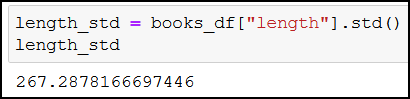
Let’s do the same for the standard deviation:

length_std = books_df["length"].std()
length_std

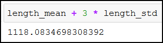
Then we calculate the values that are 3 standard deviations away from length_mean in any direction:

length_mean + 3 * length_std

And:

length_mean - 3 * length_std

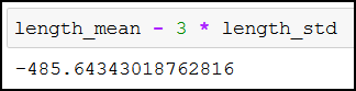
Now we can remove the outliers (data that are more than 3 standard deviations away from the mean) with the following line:

length_df_no_outliers = books_df[(books_df["length"] < 1118.0834698308392) & (books_df["length"] > -485.64343018762816)]

And finally, we can create our frequency distribution:

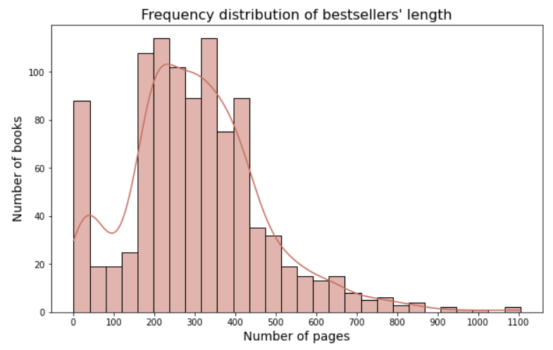
By eye, we can estimate that the length of most bestsellers is between 150-450 pages. Nice, isn’t it? 🙂

To generate the above chart, I’ve used seaborn (import seaborn as sns):

plt.figure(figsize=(10, 6))
plt.title("Frequency distribution of bestsellers' length", fontsize=16)
plt.xlabel("Number of pages", fontsize=14)
plt.ylabel("Number of books", fontsize=14)
plt.xticks(np.arange(0, 1200, step=100))
sns.histplot(length_df_no_outliers["length"], kde=True, color="#C46D5E")

Conclusion

If you’ve finished this tutorial series and have done the scraping with me, then I want you to know that I’m proud of you. It’s been no easy task, and I know it demanded a lot of time and effort on your part. Be proud of yourself, I mean it.

As a farewell gift I have something for you, a little challenge, just to stretch your newly developed web scraping muscles. Do you remember that in the books_df screenshots I had a weight and an also_available column?

Try to scrape these pieces of information, save them into a dataframe and do some analyses on them. I’m curious what insights you’ll find. 🙂 (Drop me an email if you find something interesting.)

Good luck & good scraping!

• If you want to learn more about how to become a data scientist, take my 50-minute video course: How to Become a Data Scientist. (It’s free!)
• Also check out my 6-week online course: The Junior Data Scientist’s First Month video course.

Cheers,
Tomi Mester

Cheers,

Tamas Ujhelyi