Predictive Analytics 101 – Part 2

Last week I promised to continue with the second Part of Predictive Analytics 101. If you haven’t read Part 1, please do that here: Predictive Analytics 101 Part 1.

In Part 1 I introduced the main concept of Predictive Analytics and also wrote about how predictions are useful for all online businesses. We reviewed different types of target variables, the overfitting issue, and the question of data splitting (training and test set).

At the end of this article, you will have a great overview of how Predictive Analytics works in real life! And don’t worry, this is still a 101 article; you will understand this one without a PhD in mathematics too.

Let’s continue with:

Step 4 – Pick the right prediction model and the right input values!

This is the heart of Predictive Analytics. Creating the right model with the right predictors will take most of your time and energy. It needs as much experience as creativity. And there is never one exact or best solution. It’s an iterative task and you need to optimize your prediction model over and over.

There are many, many methods. These differ mostly in the math behind them, so I’m going to highlight here only two of those to explain how the prediction itself works. If you want to go deeper, you should invest a little bit more time in that by reading some books about it, taking an online course or sneaking into a Machine Learning university class.

Anyway, as you’ve read in Part 1, there are two common cases in Predictive Analytics.

1. Answering the question “how much” with a continuous target variable (number)
2. Answering the question “which one” (aka. discrete choice) with a categorical target variable

The answer for the first question can be given by “regression” and for the second one by “classification.“

(A small reminder: we are calling the variables we are using as an input for our model predictors. They are also known as features or input variables.)

Regression

If you’ve ever used the trendline function in Excel for a Scatter Plot, then congrats! You have already applied a simple linear regression! In this model there is only one predictor and only one target variable (that’s why it’s called “simple”). The trend line tries to describe the relationship between the two.

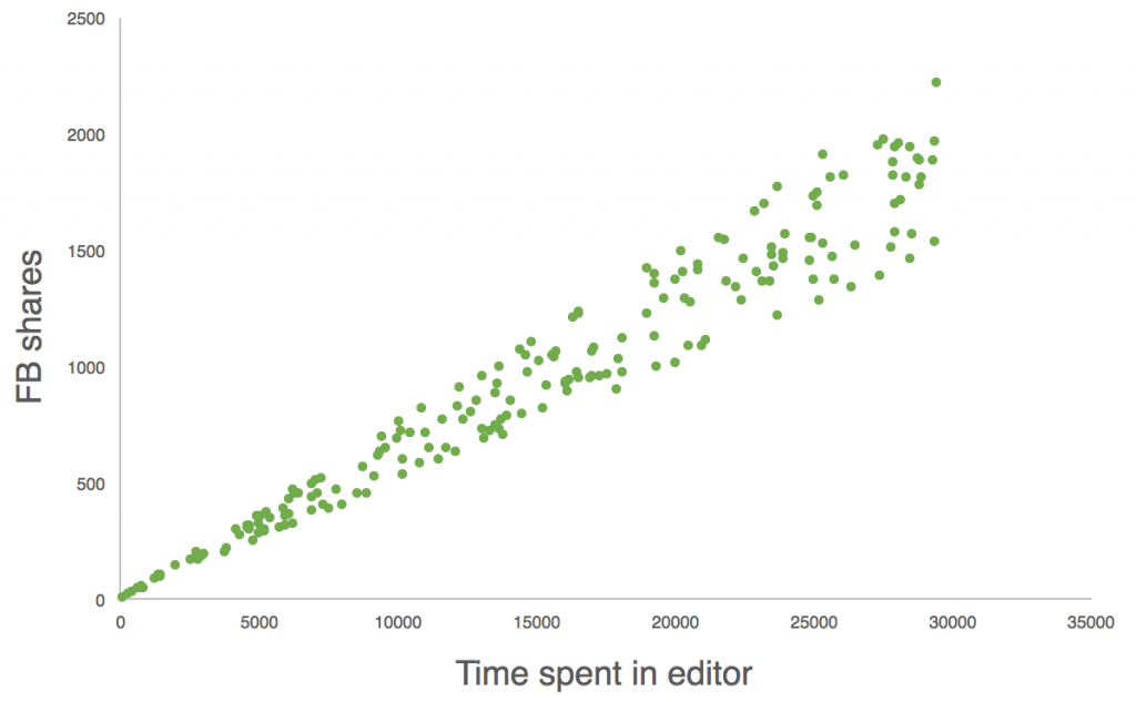
Let’s say we are running an online blogging service and we want to understand the relationship between the time bloggers spend in the text-editor and the following Facebook shares on the article. (We suspect that the more effort the writer put into the article, the better the reaction of the audience will be.) First we get the historical data (step 2) and then we split it into training and test sets (step 3). We continue with the training set. Print it on a scatter plot:

Then fit a trendline.

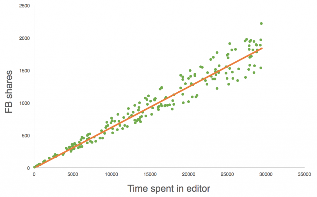
On the pictures above, we see a strong correlation between the two variables! (But remember – correlation doesn’t necessarily imply causation!) We can even go further! If someone creates a new article, we can predict the expected number of Facebook shares on that article. Of course, there is a chance that we are wrong – though we can calculate the reliability of the model too, and I’ll get back to that soon.

This method is called Simple Linear Regression because this is the simplest way to use regression. There are two ways to complicate this model:
A) Using a fitting curve that’s not just a straight line.
B) Using more than one input variable to predict the target variable.

In both cases we expect a more accurate prediction.
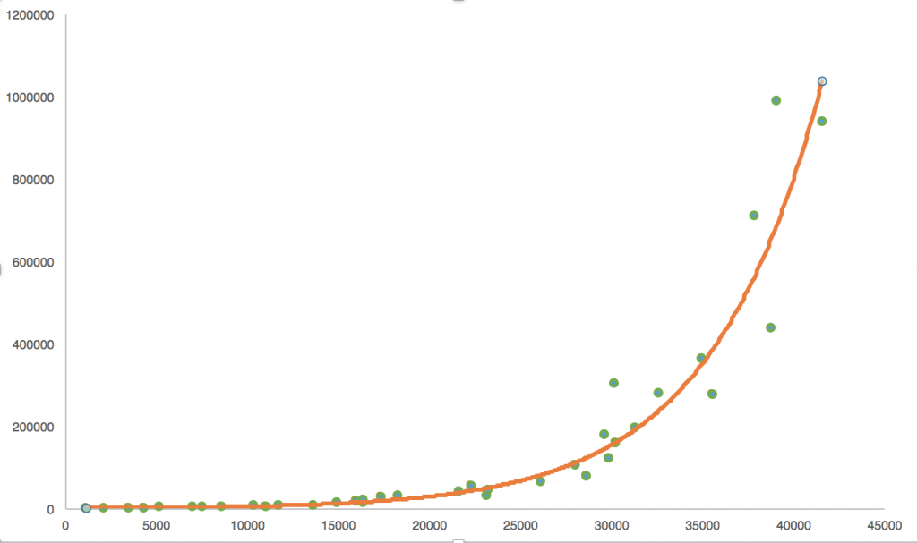
Imagine a situation where your scatter plot looks like this.

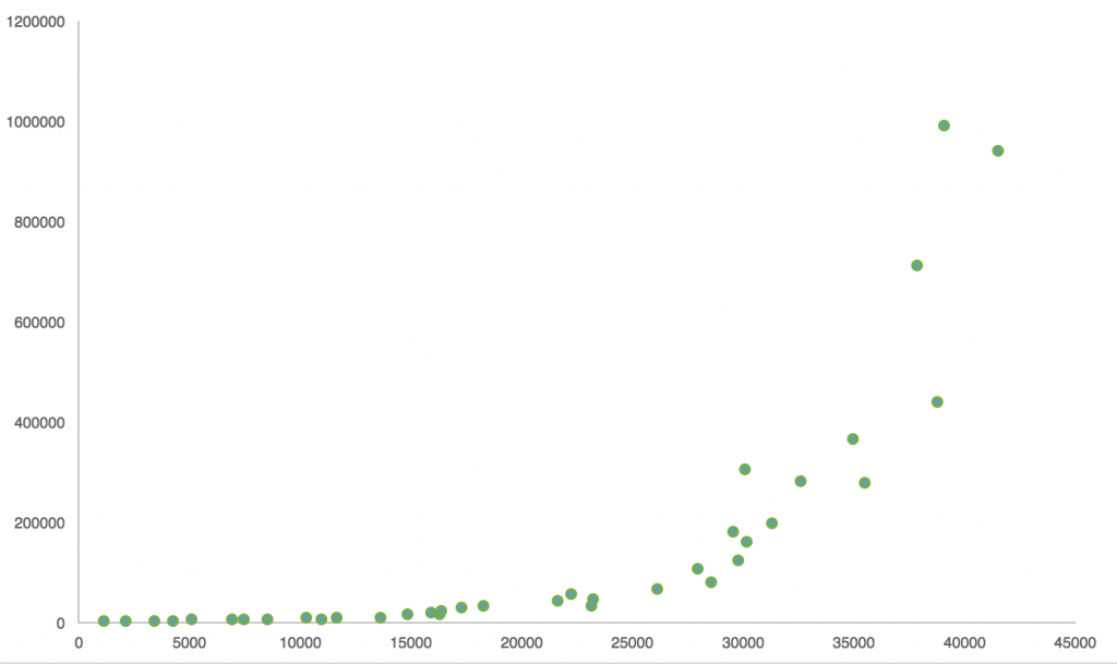
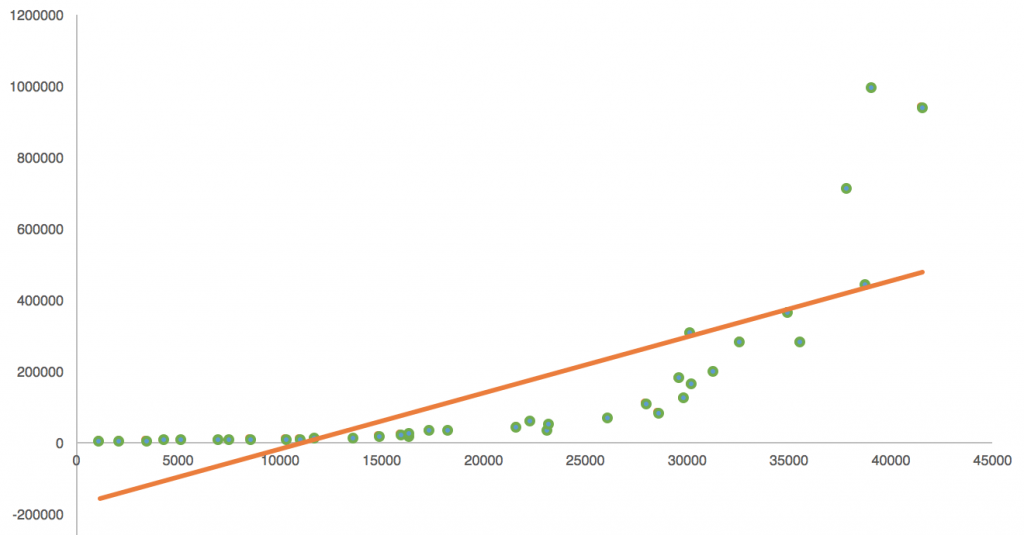
You can try to fit a straight line on it, but a curve (in this case an exponential curve) will describe the relationship between the predictor and the predicted value much better.

In real life, in most cases, you won’t use only one input value. For example, if you want to be very precise about the predicted number of Facebook shares in the above example, it’s not enough to look only at the text-editor time. You should consider bringing a few more parameters into the formula, like:

• Number of followers the blogger has
• The quality of the content (e.g. number of filler words)
• The success of previous articles written by the same blogger

Let’s pick only two for now: time spent in editor and number of followers. In this case your scatter plot won’t be a 2D graph anymore, but a 3D one. And you don’t need to assign a Y value for only one X value, but for two.

Article ID (random number)	X1 time spent in editor (predictor)	X2 number of followers (predictor)	Y number of Facebook shares (target value)
#1	1910 sec	121	100
#2	1467 sec	267	150
#3	4861 sec	12	192
#4	3218 sec	92	210
#5	…	…	…

Based on your historical data you have to predict a Y value for every possible combination of X1 and X2. Compared to the 2D one, it’s a little bit more difficult to imagine, but you can still do it by basically giving an extra dimension to everything. You scatter plot will be in a 3D space and your curve turns into a surface. It looks something like this (but hopefully with more data points).

Note: when you have multiple input values, there is a high chance that different predictors will have different weights in the formula. Weighting variables is also a big and difficult part of the job. But as this is a 101 article, let’s not go into those details.

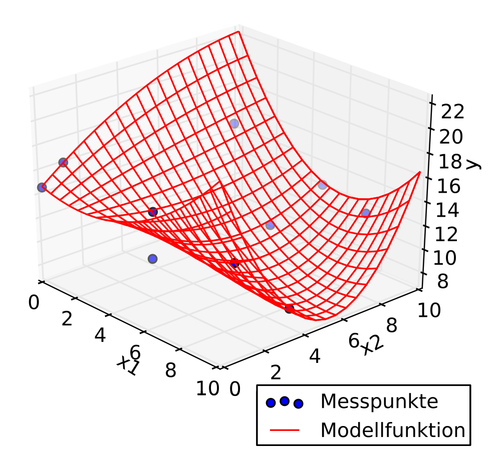
Every time you add a new feature to the formula, you should think about that as an extra dimension. Don’t worry, you don’t need to imagine the 4D, 5D, 6D spaces… computers are meant to imagine those instead of you.
The important takeaway for humans is that when it comes to regression, you should try to fit some mathematical model to your data and use that model for your predictions.

Note: There are some painful tasks you can’t avoid during a predictive analytics project. One of these is “feature reduction,” in which you remove the highly correlated or redundant variables. Another one is “feature standardization,” where you try to re-scale the different variables to make them more handy to work with.

Classification

Regression answers “how many;” classification answers “which one.” There are many classification models – an easy-to-understand one is the Decision Tree. I’m going to show you the main concept of this method!

Let’s say you are an SaaS company and you have 1,000,000 active users. You want to predict for each of them whether they will use your product tomorrow or not.

1. Your target value is a categorical value. In this example it’s a binary value (yes or no).
2. You have input values. Some of them are categorical values (e.g. paying user or not), and some of them are numerical values (e.g. days since registration).
3. Based on your historical data, you can give every categorical feature a probability value. (e.g. If the user is a paying user, then there’s a 75% chance that she will use your product tomorrow and 25% she won’t.)
4. If you have a numerical predictor (e.g. days since registration), you are trying to turn it into a categorical variable – and then give it a probability value. (e.g. if number of days since registration is lower than 100, then the chance of return is 60%; if it’s higher than 100 days, then 40%.)
5. The tricky part is that if you combine these predictors with each other, the associated probability values will change. That’s why you need the tree format, where you build a system purely from if-then statements. It will look something like this:
   

Usually, every additional level of the tree improves accuracy. The goal is to build up the tree that predicts the most accurate result in the fewest steps.

If you are done and you want to apply your model predicting if a user comes back to you tomorrow, you simply “put” the user into this tree and send it down the path of if-then statements. The result is a “yes” or “no” with X% (preferably with a high) probability.

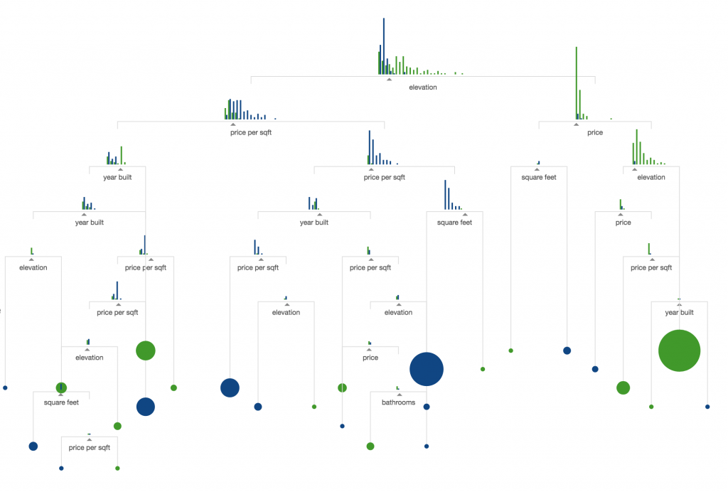
Note: maybe my description is oversimplified, but here’s another one! This is the best interpretation of Decision Tree that I’ve seen so far: the r2d3.us project. If you have an extra 10 minutes, scroll through their beautiful, highly visual learning materials!

Step 5 – How do you validate your prediction model?

In step 4 we worked with the training set to train our model! Now it’s time to use the other slice of our data to validate our model. Let’s go with the test set.
The exact process differs by prediction method, but the point is always the same: measuring the accuracy on the test set and comparing it to the accuracy of the training set. (Remember the overfitting issue!) The closer these two are to each other and the lower the percent error is, the better off we are.

Sticking with the two predictive analytics methods I described:

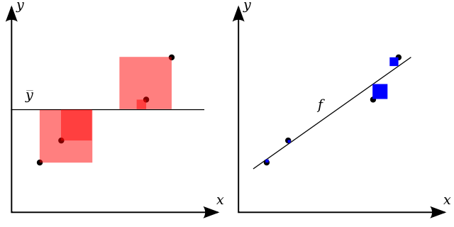
1. For linear regression, the most well-known way to measure accuracy is the R squared value. It basically tells you how well your curve fits your data and it’s calculated based on the distance between the dots and the curve. However, many professionals claim that R squared value is not enough by itself. If you want to learn more about their arguments, Google some of these: “analysis of residuals,” “confidence intervals,” and “Akaike information criterion.”
   

2. For decision trees, the case is even simpler. What you need to do is check the reality against your prediction. If you predicted yes and it’s a yes in real life, then you are good. And if you predicted yes and it’s a no, you are not good. Obviously, you won’t have 100% accuracy here, either. But that’s okay. To depict this visually, we usually put these results into a confusion matrix.

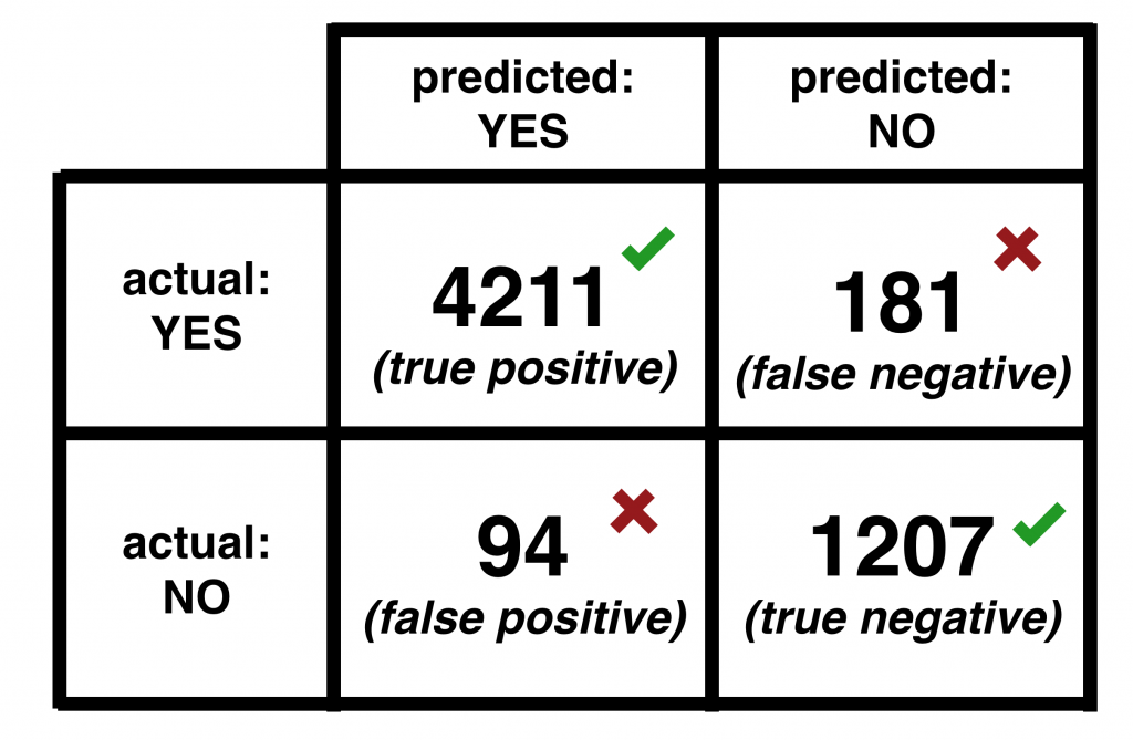
When the model correctly predicts a yes or a no, we call these values true positives and true negatives. And when the model predicts wrongly, we call them false positive and false negatives.
Accuracy = (True positive + True negative) / (True Positive + True Negative + False Positive + False Negative)
Simple, right?
Note: If you want to learn more about how to measure the accuracy of a decision tree more precisely, Google “precision and recall” or “F1 score.”

Step 6 – Implement

Yay! You are done! It’s time to start using your model to predict the future with your real-life data!

A side-note here: even if your prediction model yields pretty good results during the validation process, you should always follow-up and check back on that with the present and future data. There is a chance that you missed something during setup that messes things up when you implement your model for real.

It’s also worth mentioning that even the best prediction models start to make more and more mistakes over time, simply because life produces changes that you can never be prepared for.

All in all

To summarize the 2 articles, a predictive analytics project looks like this:

1. Select the target variable.
2. Get the historical data.
3. Split the data into training and test sets.
4. Experiment with prediction models and predictors. Pick the most accurate model.
   1. Prepare the data.
   2. Train the model on the training set.
   3. Validate it on the test set.
5. Implement it. And don’t forget to follow up on it from time to time.

When Predictive Analytics fails

Yes, Predictive Analytics can and will fail. There are two main concerns you should think about.

The first one is the same issue that Oedipus had. No, not the ‘marrying his own mother,’ but the other one: self-fulfilling prophecy. I’m going to use the online blog engine example from above. Let’s say that you clearly see from your predictions that your article will be shared more on Facebook if you spend more time in the editor. Knowing this, you can arrive at some false conclusions. Theoretically, you could type just one sentence, then leave the editor open on your computer to have a higher time-spent-in-editor value. You could click publish, and then be surprised when you realize that nobody shared it, even if you “spent” 6 hours in the editor…

We all see where the issue is. High time-spent-in-editor value is not the cause, but the symptom, of a high-quality article. The real reason is the care of the author, which causes both high time-spent-in-editor value and high number of FB shares. If you think this is a trivial issue, I can tell you: simple modelling mistakes could kill people (without quality control at least).

The other classic problem is obsolescence. Even the best models fail after a few years. There are things you simply just can’t predict. Like how could you have predicted in 2006 that, in 2016, 50% of your web-traffic would be mobile traffic? Impossible, right? Predictive models will fail by definition after a while, because you can’t prepare them for unexpected things. But that’s a known limitation. Predictive models are like cars. You should sometimes maintain or replace them.

Big Data vs. Predictive Analytics vs. Machine Learning

Just another note. I recently realized that “Big Data,” “Predictive Analytics” and “Machine Learning” are used as synonyms, though they are not. Big Data is technology to process large amounts of data (I discuss this in detail here: The Great Big Data Misunderstanding). It’s not necessarily used for Predictive Analytics nor for Machine Learning. It can be used for simple data analyses or text processing too.

I guess, if you’ve read this far, you know what Predictive Analytics is. (Basically, creating predictions based on data.) So the only question remaining is: what’s Machine Learning? In our context you can think about Machine Learning as an “improved Predictive Analytics,” where the computer automatically fine-tunes the prediction formula by learning from the difference between the predicted values and the reality.

According to Istvan Nagy, you can also think about Predictive Analytics as a business goal. In this context, Machine Learning is the approach to reach that goal, and the different models are the different tools.

Of course it’s much more than that, but then again, this is a 101 article and I don’t want to open Pandora’s box here…

Conclusion

Is Predictive Analytics easy? To understand: yes. To apply it in real life: well, I agree, it can be difficult.

My aim with these 2 articles (Part 1 here) was to highlight that it’s not rocket science. Everybody can understand the concept. And if you do, it’s only your motivation (and time, of course) that determines when you will learn the specifics and apply them in real life! Good luck, and thank you for reading!

• If you want to learn more about how to become a data scientist, take my 50-minute video course: How to Become a Data Scientist. (It’s free!)
• Also check out my 6-week online course: The Junior Data Scientist’s First Month video course.

Cheers,
Tomi Mester

Cheers,
Tomi Mester

Thank you for the early feedback on these article to:
Istvan Nagy
Laszlo Filep

Inspiration and sources:
https://medium.com/data-lab/when-is-the-best-time-to-publish-wrong-question-8f0b15be89c2
http://www.stics.com/products-and-services/sticspredicts/predictive-analysis-data-modeling/
http://www.r2d3.us/visual-intro-to-machine-learning-part-1/
http://www.martingoodson.com/ten-ways-your-data-project-is-going-to-fail/
https://en.wikipedia.org/wiki/Linear_regression
https://en.wikipedia.org/wiki/Regression_validation