
This article is about dating and data science!
Please welcome our guest author, Amy Birdee, who has done multiple data science hobby projects recently and built a truly awesome portfolio. Amy’s Github is just the perfect example of how one should demonstrate their skills as an aspiring data scientist… No surprise that Amy got hired as a Lead Data Analyst recently. Amy’s guest post is about how she has done exploratory data analysis using the OkCupid Dataset. Enjoy!
The project: OkCupid Data + Python
After finishing Tomi’s six-week Junior Data Scientist course, I couldn’t wait to start using my new skills and exploring data on my own. I knew that if I wanted to make a career transition into data analytics/data science, I had to build my own portfolio of hobby projects and this article talks through one of those projects.
Customer data is always quite fascinating no matter what industry you are in. For this project, I chose the dating industry and conducted an exploratory data analysis of the OkCupid profile database. The dataset includes circa 60,000 members of the dating site with features such as age, height and their eating and drinking preferences (well these things are all important when you’re trying to find a match right?!).
The project was carried out in Python, so if you haven’t already done so, I would recommend you first read Tomi’s Learn Python for Data Science – from scratch series.
If you’d like to follow along, you can download the data from my github or you can just use this as a guide for your own data projects. This article is in two parts – part 1 explains how I explored and cleaned the data and part 2 [coming soon…] describes how to visualise the data with three different chart examples.
Import the libraries and view the data
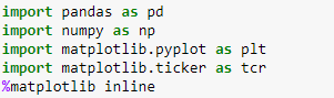
Ok so let’s get started. First, import the libraries. We will need:
pandas– for manipulating data frames and extracting datanumpy– for calculations such as mean and medianmatplotlib.pyplot– to visualise the datamatplotlib.ticker– to make the chart labels look pretty
…and then read in the data. We will save the data file to a variable called ‘dating’.
dating = pd.read_excel('/home/amybirdee/hobby_projects/dating_site/profiles.xlsx')
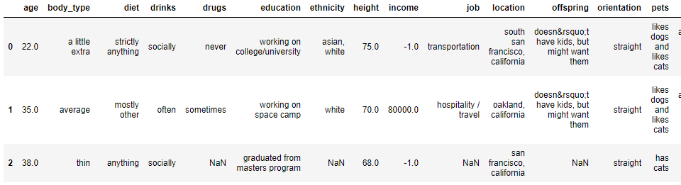
Once this is done, we can use the dating.head(3) command to view the top two rows of data.
This is what we get:
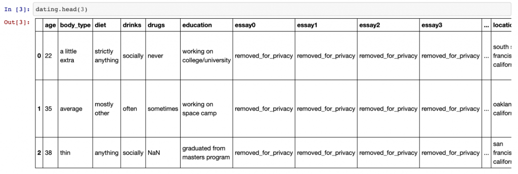
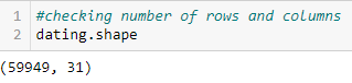
As you can see, there are quite a few columns (too many to fit into one screenshot). Using the .shape command — which gives the shape of the data frame — we can see there are 31 columns in total and 59,949 rows.
Data exploration
Identifying data cleaning issues
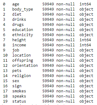
So now we know the shape of our data file, which is great, but more information would be even better. So next we will look at the file information using the command dating.info(). This gives us the following useful table:
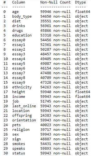
Here we can see all our column names as well as the number of entries for each column and the data type. We know we have 59,949 rows in our file… but none of the columns in the above table have this many entries. This means our file contains missing data which we will need to deal with as part of the data cleaning process.
It’s good to see that the age, height and income fields are already in a numeric format. Although since they are floats, they will be in decimal format and we will convert them to integers later on — as this will look neater in the charts.
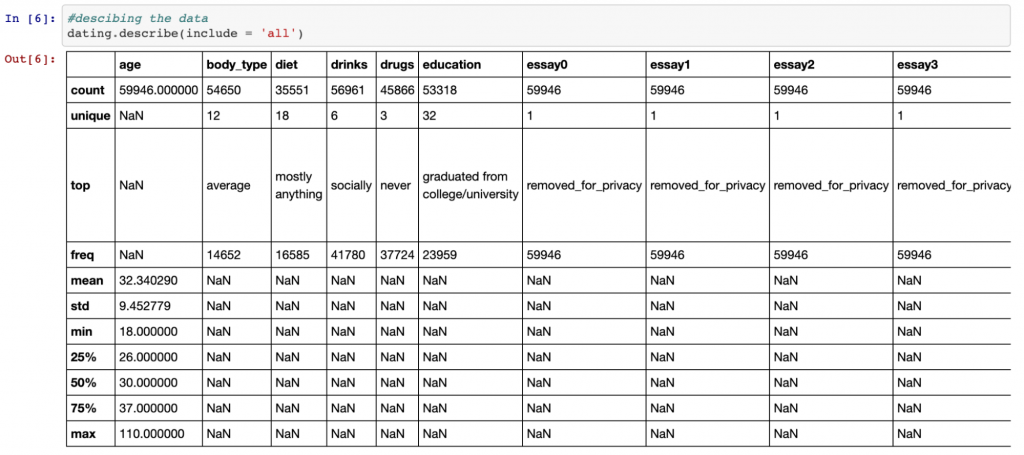
Another great function for exploring data is the describe() function. If we also include the ‘all’ parameter, this will give us information about the categorical variables as well as the numeric variables as shown below.
dating.describe(include = 'all')
Different data types, different data cleaning techniques
For numeric variables, the describe() function provides details of the mean, standard deviation, the min and max values and the quartiles. For categorical values, it gives details of the most common value and how many unique values there are. This is valuable information as it can give us an idea of how we would like to deal with null (missing) values.
For example, we can see that the mean age is 32, with the minimum value being 18 and the maximum 110 (hey, you’re never too old to start dating!). The fact that the mean is so much lower than the maximum suggests that the distribution of the age data is skewed to the right (i.e. it has a long tail to the right – we will see this in a chart in part 2). Therefore, since this isn’t a normal distribution, it may be better to fill null values with the median value (the middle value) in this case rather than the mean.
Similarly, for categorical values, the majority of OkCupid members have classed their body type as ‘average’. Since this is likely similar to the wider population, we may decide to fill all missing values in this column with ‘average’.
The columns we won’t need
Now, there are a few columns in our data file which we will not be using in this analysis. These are the essay columns and the last_online column. The essay columns contain free text in which the members write a description about themselves and the last_online column shows when the users were last online. Given that each user is unique in our data, this column won’t be of much use to us. To drop these columns, use the following line of code:
dating = dating.drop(['essay0', 'essay1', 'essay2', 'essay3', 'essay4', 'essay5', 'essay6', 'essay7', 'essay8', 'essay9', 'last_online'], axis = 1)
More issues
If we review our data frame again using the dating.head() command, you can see that it looks a little better but there is still more work to do – we still have missing values to deal with, integers are incorrectly expressed as floats and Python clearly hasn’t read the ‘offspring’ column correctly so that’s another issue!
Data cleaning
Filling in empty values — with fillna()
First let’s fill in the null values which show up as ‘NaN’ in Python. For the reasons described above, I decided to fill the age column with the median and the body_type column with ‘average’. For the height and income columns, I chose the mean as the fill value. For height this was because I assumed height would be normally distributed (I was right!) and for income, the mean was just an arbitrary value – the majority of this column is filled with a value of -1.0 which is meaningless so the data will not be helpful in our analysis regardless of whether we use the mean or the median as a fill value.
For all other categorical values, the fill value used was ‘no response given’ because I didn’t have enough information to fill the values in any other way and didn’t want to introduce any bias.
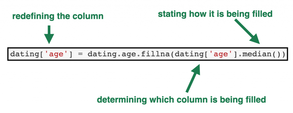
Below is some example code showing how the fillna() command works:
dating['age'] = dating.age.fillna(dating['age'].median())
- The first part of the code,
dating[‘age’] =tells Python we are redefining theagecolumn in the dating table. - The
dating.age.fillnapart tells Python the column in which the null values are being filled. - And the part in the brackets —
(dating['age'].median())— shows which value to use as the fill value – in this case the median of theagecolumn in thedatingdata frame.
Similarly, we can also use other fill values as follows:
dating['height'] = dating.height.fillna(dating['height'].mean())
dating['body_type'] = dating.body_type.fillna('average')
dating['diet'] = dating.diet.fillna('no response given')
As you can see, using the mean as the fill value is pretty similar to the median – we just use .mean() instead of .median(). For categorical values, it’s just a case of putting the string we want to fill with in quotation marks.
Converting floats to integers — with astype()
Once every null value has been filled in all columns, we can move on to converting the floats to integers. There are only three columns to convert – age, height and income – and the code is as follows:
dating['age'] = dating.age.astype(int)
dating['height'] = dating.height.astype(int)
dating['income'] = dating.income.astype(int)
As you can see it is just a case of redefining those columns once again and converting them (using the astype() command) to integers.
Fixing character encoding issues — with replace()
Finally, there are two columns where Python has read the data incorrectly – these are the offspring and sign columns. Looking at these columns closely, it seems that Python has read the apostrophe in the word doesn’t and converted it into a nonsensical string: ‘’’.
(Comment by Tomi Mester: That’s actually some sort of ASCII encoded version of the apostrophe character. This could be useful in HTML projects. Guess that’s how it’s ended up in this dataset, as well.)
It makes sense that Python didn’t read the apostrophe correctly because these are usually used at the start and end of a string. In this case, however, the apostrophe formed part of a word and Python handled that as best it could. If the apostrophe had had a backward slash (\) immediately before it, Python would have known to ignore it and would have read the data correctly but alas that was not the case here.
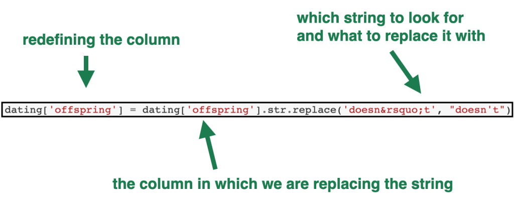
But we can easily clean these two columns with the following code:
dating['offspring'] = dating['offspring'].str.replace('doesn’t', "doesn't")
dating['sign'] = dating['sign'].str.replace('doesn’t', "doesn't")
Here we have used the str.replace() command to replace the incorrect word with the correct word. The diagram below breaks down each part of the code.
Data cleaning: done!
Now when we look at our data frame information again using the .info() command we see the following table:
- Now we only have 20 columns of data (since we removed the unnecessary columns),
- our numeric columns are now integers rather than floats and
- we have no null values
Fantastic!
We can now start visualising the data which we will do in Part 2. Stay tuned, it’s coming soon…
Cheers,
Amy Birdee